How a hologram records and replays light
A hologram is a diffraction grating that a wave wrote into a plate: record the interference of an object wave and a reference beam, and the developed fringes bend a fresh beam back into the original wave.
1. What a hologram stores
Hold up a real object and look at it. Each eye catches the light coming from every visible point, each ray arriving at its own angle, and the brain reads those angles — and the way they shift as you move — as solid depth. The object itself never reaches you; only the light it sends does. So if a flat surface could emit exactly that light — the same rays, in the same directions, at the same brightness — an eye in front of it would see the object in full depth, with nothing there. That is the aim of holography: not to photograph a scene, but to store and replay the whole field of light it sends.
The obvious way to build that is ray by ray. Tile the surface with tiny emitters and have each one send light out in the exact fan of directions the scene would have. This is a light-field display, and it works — poorly. To aim a beam into a chosen direction, or to make it appear to spring from a point at a chosen depth, you have to control the light across an aperture at the scale of its own wavelength, about half a micron. Doing that independently at every point of a panel would take billions of separately steered elements; settling for coarse pixels gives the thick, narrow-angle, jagged 3-D of a lenticular postcard. Synthesizing the ray field by force runs straight into the wavelength.
The escape is to stop counting rays. A ray is only bookkeeping — the local direction in which a wave is heading. The light leaving the scene is one continuous wave: a single surface of crests and troughs sweeping outward, with the rays no more than its perpendiculars. Re-create that one wave where it crosses a plate and you have re-created every ray at once — every direction, every viewing angle, the slightly different view each eye needs, all together. The impossibly-many-rays problem collapses into a single object: the wave at the plate.
Ray by ray. Fling light from every pixel into every direction the scene needs, each beam aimed and focused to a fraction of a wavelength. A whole panel of them is the brute-force display — and steering light that finely, everywhere, is punishing.
One wavefront. A ray is just the local direction a wave travels — its perpendicular (green). Re-create the single wave crossing the plate and every ray, every viewing angle, the distinct view at each eye, follows for free.
And that object stays simple however busy the scene is. Every point of the object adds its own small wave to the plate, and waves add: the total is their sum. A sum of waves of one colour is again just a wave of that colour, so at each point of the plate the whole scene comes to a single crest height and a single timing — one amplitude and one phase. To store a scene in depth is to store, across the plate, only those two numbers at every point. That is the entire target.
One of the two is easy and the other is nearly impossible. Amplitude is just brightness, which any film or sensor records. But phase — the timing of the crests, the number that actually carries direction and depth — rides an oscillation at hundreds of terahertz. No detector is remotely that fast; each only reports how much light arrived, averaged over the exposure, and the phase averages to a smooth glow. A plain photograph of the object wave keeps the easy number and loses the one that matters.
The wave a point sends — the shape of the arriving wavefront, the timing of its crests, is the phase: that is what tells the eye where the point sits in depth.
A plain exposure of it — a smooth, featureless strip. Recording intensity keeps the brightness and throws away the shape, so none of the geometry survives.
The trick is not to measure the phase but to convert it into something a detector does keep — brightness. Add a second wave: a reference beam, split from the same laser that lights the object, and let the two interfere at the plate. Where they arrive in step the intensity is high; where they arrive half a cycle apart it is low. The positions of the resulting fringes are set by the phase difference between the object wave and the reference, so an ordinary intensity recording of the fringes stores the phase after all. The developed plate is a diffraction grating that the object wave itself wrote; lit by the reference again, the grating diffracts the beam into a copy of the original object wave.
Because that pattern is simply the sum over the scene, it holds every point at once. Lit again by the reference, the plate regenerates the whole wavefront in a single step, and any eye in front of it receives exactly the light the original scene would have sent — at any viewing angle, and a different view at each eye, which is what makes it look solid. Notice what the interference bought: structure in the plate at the scale of the wavelength — the very fineness the ray-by-ray display could not manufacture — laid down for free by letting the object wave carve it. Everything below is that one idea, turned one knob at a time.
The figures are live. Each embeds the same 2D wave-optics simulator (full version here): a horizontal slice of the classic off-axis (Leith–Upatnieks) setup, with point sources standing in for the object, a vertical film plate, and a plane-wave reference tilted by \(\theta_R\). You can drag the sources (and, later, the eye) in every figure, and the dashed-underlined “try it” links throughout set the figures to specific demonstrations.
2. Two waves interfere
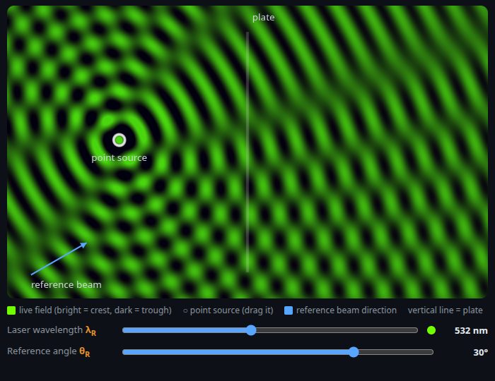
Figure 1 shows the instantaneous field: the object wave and the reference added together, animated in time. Each point source emits a circular wave (a cylindrical wave, in this 2D slice) whose amplitude falls off as 1/√d; the reference is a plane wave arriving at \(\theta_R\) from the plate normal. Bright is a crest, dark a trough.
Both waves come from one laser, so they share a single frequency, and the pattern of reinforcement and cancellation is stationary: the crests march, but the places where crest reliably meets crest — and the places where crest always meets trough — stay put. Along the plate this stationary pattern is a set of interference fringes whose local spacing depends on the angle between the two waves at each height. The stationary pattern, not the marching field, is what the plate can record.
3. The exposure records the pattern
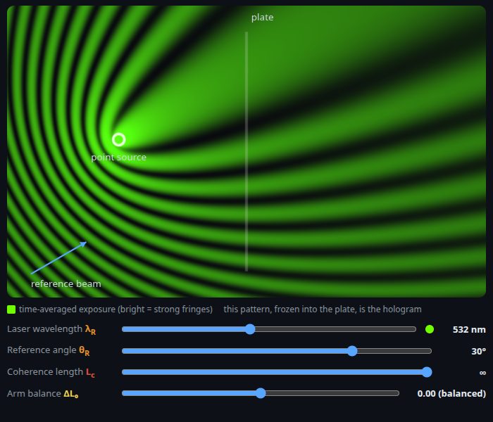
Film cannot follow a field oscillating at hundreds of terahertz; it integrates. Figure 2 shows the time-averaged intensity over the exposure. The traveling crests average out, and the stationary interference pattern of section 2 survives: bright bands where object and reference stay in step, dark bands where they stay opposed.
This frozen pattern is the hologram. Developed into the plate it becomes a transmittance t(\(y\)) — a physical grating, with the recording geometry encoded in its fringe spacing and contrast. Nothing else is stored: there is no lens in the system and no image anywhere on the plate.
4. The plate is a grating
From here on, the equations use a consistent color code:
Color code, used in every equation below — recording beam: \(\lambda_R, \theta_R\) · replay beam: \(\lambda_P, \theta_P\) · their ratio \(\mu =\) \(\lambda_P\)/\(\lambda_R\) · geometry: \(y, d, a, b, \theta_{\mathrm{obj}}, \Delta L\) · diffraction order \(m\) · noise: \(\sigma_\lambda, \sigma_\theta, L_c\). The same few groupings recur: every image property is geometry scaled by \(\mu\) and shifted by the replay–recording mismatch.
The same few symbols recur throughout. This table pairs each with its meaning and with the control that sets it, in the figures and in the full simulator:
| \(\lambda_R\) | recording (laser) wavelength — sets the fringe spacing written into the plate | Laser wavelength |
| \(\theta_R\) | reference-beam angle at recording, measured from the plate normal | Reference angle |
| \(\lambda_P\) | replay (reconstruction) wavelength | Replay wavelength |
| \(\theta_P\) | replay-beam angle | Replay angle |
| \(\mu\) | = \(\lambda_P\)/\(\lambda_R\), the wavelength ratio that scales every image position | (derived) |
| \(y\) | height up the plate; \(\theta_{\mathrm{obj}}(y)\) is the object-ray angle there, \(d\) its path length | — |
| \(a, b\) | a source sits at (\(-a, b\)): depth \(a\) in front of the plate, height \(b\) | drag on canvas |
| \(H\) | plate half-height = half the aperture; sets resolution \(\sim\) \(\lambda\)\(/2H\) | Plate half-height |
| \(D\) | distance the eye is focused (accommodated) to | Eye focus distance |
| \(m\) | diffraction order: 0 = straight through, +1 = image, −1 = conjugate twin | — |
| \(L_c\) | coherence length — how far apart two path lengths can be and still make fringes | Coherence length |
| \(\Delta L_0\) | delay-line detuning — extra reference path beyond the length that balances the arms (to source 1) at the plate center | Arm balance |
| \(\sigma_\lambda, \sigma_\theta\) | recording jitter: laser linewidth and reference-angle wobble during exposure | Wavelength / Angle jitter |
| \(\sigma_L, \sigma_g\) | path-length (vibration) jitter and additive plate-grain noise | Phase jitter / Plate grain |
| \(\sigma_{\lambda P}, \sigma_{\theta P}\) | replay-source spread: bandwidth (LED vs laser) and angular diffusion (lamp vs point) | Replay bandwidth / diffusion |
Recording stores fringes whose local spacing depends on the angle mismatch between the object ray and the reference at each plate height y. On replay, each little patch of plate diffracts the replay beam into three orders, m = 0, ±1:
where \(\theta_R\), \(\lambda_R\) are the recording reference angle and wavelength, \(\theta_P\), \(\lambda_P\) the replay ones, and sin \(\theta_{\mathrm{obj}}\)(y) = (y − \(y_s\))/d is the direction of the object ray that hit the plate at \(y\). Note the bracket is pure recording geometry — it is what the plate stores; the replay terms only scale and shift it.
The plate stores lengths: the local fringe spacing is set at recording time and never changes afterwards,
The simulator’s live analysis panel draws the fan of orders and the recorded t(\(y\)) strip for whatever the sliders currently say, alongside the worked numbers used in this article.
5. Replay: one beam in, three waves out
Zero order (m = 0): the undiffracted beam
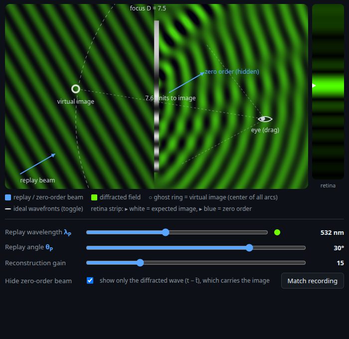
The replay beam passing straight through, attenuated by the average transmittance t̄. Mind the amplitude–power distinction here: the wave keeps a fraction t̄ of the incident amplitude, so its power is t̄² — about 28% at the default t̄ ≈ 0.53 — and the largest share of the incident power is actually absorbed in the dark fringes of the plate. A thin amplitude hologram diffracts at most 6.25% = 1/16 of the incident power into each first order, reached when the fringe swings the full 0–1 range; the live bar in the simulator shows the current values — 1/16 is the ceiling. The zero order contains no image information. How deep the fringes swing is set by how close the object and reference amplitudes are at the plate; here the reference amplitude is fixed at \(A_{\mathrm{ref}}\) = 0.7 and the object falls off as 1/√d, so contrast is good near the source and fades with distance. Hiding the zero order leaves exactly the information-bearing part Δt = t − t̄.
Figure 3 hides the zero order by default (“Hide zero-order beam”) — show the full field to see the image wave ride beneath the replay beam.
Where the energy goes
The budget is an exact Parseval split of unit incident power for a thin amplitude hologram, illuminated at unit amplitude across the aperture with obliquity ignored: the zero order carries t̄², the two sideband families (all m > 0 and all m < 0) carry ⟨Δt²⟩/2 each, and the remainder, 1 − ⟨t²⟩, is absorbed by the plate — for typical fringes the largest share. With several recorded sources the sideband families also include the intermodulation (object–object) terms, not just the ±1 images. When the −1 order is evanescent (drawn hatched in the live bar) its share is not radiated and is not handed to the other orders: it is dissipated at the plate.
The simulator’s live analysis panel computes this split — absorbed, zero order, +1, −1 — from the current plate as you move the sliders.
6. The virtual image (m = +1)
The regenerated object wave. With matched replay (\(\lambda_P\) = \(\lambda_R\), \(\theta_P\) = \(\theta_R\)) the grating equation returns \(\sin\theta_{\mathrm{out}}\) = \(\sin\theta_{\mathrm{obj}}\) exactly, at every plate point: the wave continues as if the object were still there. It never appears as a bright spot in the field — it is the common center of curvature of the arcs. An eye must focus the diverging bundle to “see” it (the retina strip in Figure 4 does this). For a source at (\(-a, b\)) and \(\mu\) = \(\lambda_P\)/\(\lambda_R\), paraxially:
Derivation
For a source at (−\(a\), \(b\)), the distance from the source to the plate point (0, \(y\)) is
— the Fresnel (paraxial) expansion. The plate’s ±1 components store the phase ±[\(k_R\) \(d(y)\) − \(k_R\) \(y\) sin \(\theta_R\)], and the replay beam adds \(k_P\) \(y\) sin \(\theta_P\), so the \(m\) = +1 wave leaves the plate with phase (constants dropped)
Compare this with a wave diverging from an image point at depth R behind the plate and height \(y_i\), whose phase on the plate is \(k_P\)(\(y\) − \(y_i\))²/2R + const. Matching the \(y\)² coefficients gives \(k_P\)/2R = \(k_R\)/2\(a\), so R = \(a\)·\(k_P\)/\(k_R\) = \(a\)/\(\mu\) (since \(\mu\) = \(\lambda_P\)/\(\lambda_R\) = \(k_R\)/\(k_P\)). Matching the \(y\)¹ coefficients gives −\(k_P\) \(y_i\)/R = \(k_P\) sin \(\theta_P\) − \(k_R\) sin \(\theta_R\) − \(k_R\)\(b\)/\(a\), which solves to \(y_i\) = \(b\) − (\(a\)/\(\mu\))(sin \(\theta_P\) − \(\mu\) sin \(\theta_R\)) — the formula above.
The \(m\) = −1 component carries the recorded phase with the opposite sign, so its quadratic coefficient is −\(k_R\)/2\(a\): a converging wave, i.e. a real focus at x = +\(a\)/\(\mu\), and the same linear-term matching gives \(y_c\) = \(b\) + (\(a\)/\(\mu\))(sin \(\theta_P\) + \(\mu\) sin \(\theta_R\)) — the conjugate formula in the next section.
This expansion is what “paraxial” means here: for large angles or sources close to the plate the neglected terms of \(d(y)\) no longer cancel, and they appear in the applet as the aberrations that grow with detuning.
The +1 wave leaves the plate diverging, as if from a point behind it — the common centre of curvature of the arcs. Nothing is there and no screen can catch it, but the eye traces the bundle back (dashed) and sees a point: a virtual image.
Longer replay wavelength (\(\mu\) > 1): the image pulls toward the plate and shifts — holographic dispersion, the reason white-light transmission holograms smear into rainbows. Detuned replay angle: the image translates with sin \(\theta_P\), and because the formula is only paraxial, large detuning also aberrates it — watch the arcs stop matching the ideal rings. The dashed “predicted image” marker shows this position whenever it differs from the recorded source.
7. The conjugate image (m = −1) and evanescence
The phase-reversed twin: where the +1 order diverges from the virtual image, the −1 order converges, forming a real, pseudoscopic (depth-inverted) image on the observer side:
The same fringes produce both images. The +1 wave diverges from a virtual point behind the plate (upright, un-catchable). The −1 wave converges to a real point in front — you can catch it on a card, but it is depth-inverted (pseudoscopic). Off-axis recording throws the twin to a different angle so only one is seen.
Wherever the grating equation gives \(|\sin\theta_{\mathrm{out}}| > 1\) the order is evanescent — it decays within about a wavelength of the plate and radiates nothing. At the default 30° reference nearly all conjugate rays are evanescent (check the toggle), which is the point of off-axis holography: Leith and Upatnieks tilted the reference precisely so the three orders separate in angle. Re-record at ≤15° and the conjugate propagates, overlapping the image — Gabor’s original in-line problem.
Evanescent orders: what “\(|\sin\theta| > 1\)” means
A wave leaving the plate has a transverse wavenumber \(k_y = k\sin\theta_{\mathrm{out}}\) and a forward one \(k_x = k\cos\theta_{\mathrm{out}}\), tied together by \(k_x^2 + k_y^2 = k^2\). The grating can push \(k_y\) past \(k\) — the diffracted direction would need \(|\sin\theta_{\mathrm{out}}| > 1\), which no real angle satisfies. Then \(k_x = k\sqrt{1 - \sin^2\theta_{\mathrm{out}}}\) turns imaginary, and that order becomes evanescent:
It clings to the plate surface, decays within about a wavelength, and carries no power to the far field. Its share of the energy budget is not handed to the other orders, either: in an amplitude hologram the order amplitudes are fixed Fourier coefficients of t(y), so the power an evanescent order would have carried is dissipated at the plate. (Only in a lossless phase grating, which cannot absorb, must that power redistribute among the propagating orders.) So an “evanescent conjugate ray” is a conjugate (−1) direction the grating tried to send past 90°: at a steep reference angle the conjugate is bent so hard it can’t propagate, which is exactly what lets off-axis holography show a clean single image. The simulator’s live order-fan diagram draws any evanescent order as a decaying squiggle instead of a ray, and the conjugate toggle in Figure 3 reports how many of its rays are evanescent.
Propagating — the wavefronts tilt and march off the plate, carrying energy to the observer.
Evanescent — the crests lie flat against the plate and the amplitude decays within about a wavelength: no ray leaves, no energy reaches you.
8. Higher orders
The grating equation allows any integer \(m\), so why only three orders here? Because a thin, linearly recorded hologram stores a single cosine fringe: t(y) = t̄ + \(t_1\)cos(2πy/Λ). A pure cosine has only the spatial frequencies 0 and ±1/Λ — so it can only make \(m\) = 0, ±1. Higher orders need higher harmonics in the transmittance, which appear only when recording is nonlinear: overexposure clipping, a development curve with γ ≠ 1, or a squared/thick response. Then t picks up cos(2·2πy/Λ), cos(3·…)… and orders \(m\) = ±2, ±3 fan out at \(\sin\theta_{\mathrm{out}}\) = sin \(\theta_P\) + \(m\)·\(\mu\)·[…], each a fainter, more strongly dispersed copy of the image (and each evanescent once \(m\)·μ bends it past 90°). This sim keeps recording linear, so those harmonics have zero amplitude — the simulator’s live order fan marks where \(m\) = ±2 would emerge with a faint dotted ray, but no light goes there. (Emulsion grain and the plate’s Δt noise are a different, incoherent kind of extra light — haze, not sharp orders.)
Linear recording — the fringe is a pure cosine; its spectrum is only 0 and ±1. Three orders only.
Nonlinear recording (clipping, γ ≠ 1) — flat-topped fringes carry harmonics, so ±2, ±3 orders fan out. This sim stays linear, so they don’t.
9. Replay wavelength sets the image geometry
Section 4 made the point that the plate stores lengths: the fringe spacing Λ(\(y\)) was fixed at recording time.
On replay, every diffraction effect is the ratio of the light to those stored lengths: the local deflection is \(\sin\theta_{\mathrm{out}}\) − sin \(\theta_P\) = \(m\)\(\lambda_P\)/Λ(\(y\)), so longer replay light is bent harder by the same plate. Through the paraxial formulas this gives the wavelength mismatch a very specific geometry:
With plane-wave reference and replay, two recorded points at different heights stay the same distance apart in the image for any \(\mu\) — but their depths compress by 1/\(\mu\). So replaying green-recorded fringes with red light (\(\mu\) > 1) doesn't zoom the image, it flattens it (and shifts it, per the position formulas above); blue replay stretches it. Wavelength mismatch is a shape distortion, not a magnifier. Sizes of everything diffraction-limited scale with \(\lambda_P\) too: the image spot through the plate aperture A blurs by δθ ≈ \(\lambda_P\)/A, the eye's resolution is \(\lambda_P\)/W, its depth-of-field threshold 2\(\lambda_P\)/W², and the ideal-wavefront rings are spaced \(\lambda_P\).
Replay a three-point scene at 650 nm on Figure 3: the dashed marker shows the first source’s image pulled toward the plate, displaced from where it was recorded.
Matched replay (\(\mu\) = 1) — the recorded shape comes back true, full depth.
Longer replay (\(\mu\) > 1) — same width, but depths squashed by 1/\(\mu\): the scene flattens toward the plate.
Numerically validated: across 450–650 nm replay the actual reconstructed wave's center of curvature matches the dashed paraxial marker to ≤0.12 units transversely; the longitudinal position agrees within ±0.4 units, which is the depth-of-field limit itself — through a finite aperture, depth is only defined that precisely. One caveat for real holograms: this plate is thin, so it diffracts any color you send at it. Thick (volume) holograms add Bragg selection along the plate's depth, which is why a Denisyuk reflection hologram picks its own color out of white light.
10. Aperture: the plate is a window
The plate is the hologram’s aperture, and like any aperture its width A = 2H sets the diffraction-limited resolution of the reconstruction:
A larger plate captures a wider cone of each object wave, records more fringes, and reconstructs a sharper image with a wider viewing zone — a hologram really is a window, and the plate is the window frame. A smaller plate intercepts only a narrow slice of each spherical wave, so the reconstruction blurs and the parallax shrinks; in the limit of a plate a few fringes wide it barely diffracts at all. This is the same 1/aperture scaling as the coherence-length knob, except that limits the effective aperture through fringe visibility while this sets the physical one. (The plate is always sampled at 2048 points, so the finest fringe stays well resolved across the whole size range.)
Small plate — only a narrow cone of each wave is caught, so the image point spreads (δθ ≈ \(\lambda\)/A is large) and the window is tiny.
Large plate — a wide cone is caught, more fringes are recorded: a tight sharp point and a wider window to look around the scene.
Zoom (view span) is not an aperture
“Zoom out” changes nothing physical — not the plate size, the wavelength, or the fringe spacing. It only widens the viewport, so the plate (a fixed object of half-height 3 units) fills less of the frame and you watch the waves propagate further out. It is exactly stepping back from a real hologram: the reconstructed image subtends a smaller angle and looks farther away, and because more wavelengths now fit across the frame the fringes look finer. Markers, the plate line, and arrows keep a constant screen size so they stay readable; all measured distances (e.g. “7.6 units to image”) are in fixed scene units and do not change with zoom.
11. Seeing the image: the eye
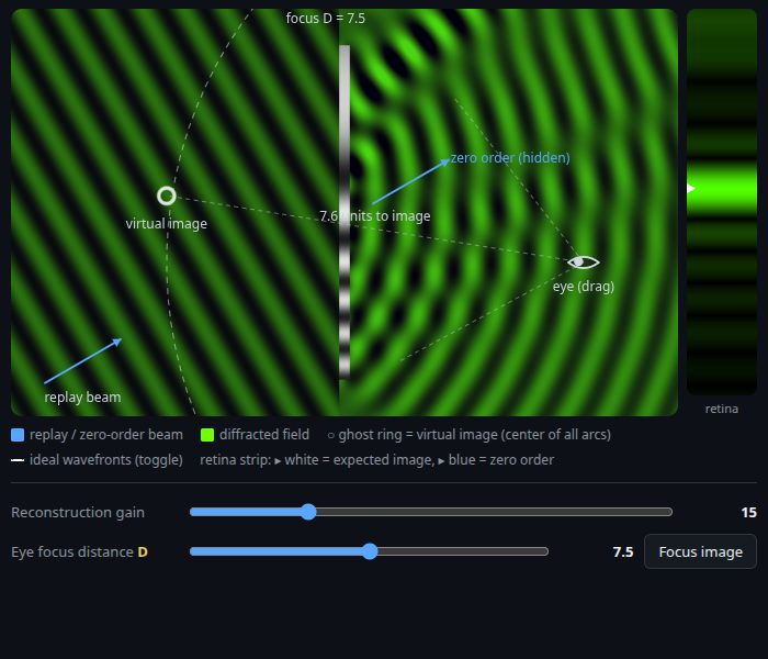
A virtual image cannot be caught on a screen; something has to focus the diverging bundle. The simulator’s observer is a one-dimensional eye: a pupil of width W = 6 units, a lens accommodated to a distance \(D\), and a retina strip that scans across its field of view.
The retina intensity at gaze angle α is a focus scan:
A lens focused at distance D maps each direction to a retinal point; the response peaks when F lands on a wave’s center of curvature. The strip is normalized to the ideal-focus response, so accommodation is visible as brightness: sweep D through the measured image distance and the spot swells to full brightness, then dims again. Two honest caveats. First, the spot’s direction barely moves with focus — a misfocused eye still receives light from the image direction, just spread out; direction is the robust observable, depth is a soft one. Second, depth of field: misfocus only registers when the wavefront-sag difference across the pupil exceeds ~a quarter wave,
With the giant λ of this toy world a 3-unit pupil could not distinguish the image distance from infinity (threshold 0.14 vs 1/\(D_{\mathrm{img}}\) ≈ 0.13) — hence the 6-unit pupil, which gives ~16% response at D = 4, 100% at \(D_{\mathrm{img}}\), ~18% at D = 30 in the default geometry. The zero-order beam (blue marker) stays bright at any focus: a plane wave has no curvature center to accommodate on.
On Figure 4, pull the focus in to D = 4: the spot dims and spreads without leaving its direction. “Focus image” snaps back to the measured image distance.
12. Imperfections
Everything so far assumed an ideal exposure and an ideal replay source. Each departure has a specific, recognizable signature, and almost all of them act through one quantity: the fringe visibility V — the contrast the moving interference pattern manages to leave in the plate.
12a. Coherence and arm balance
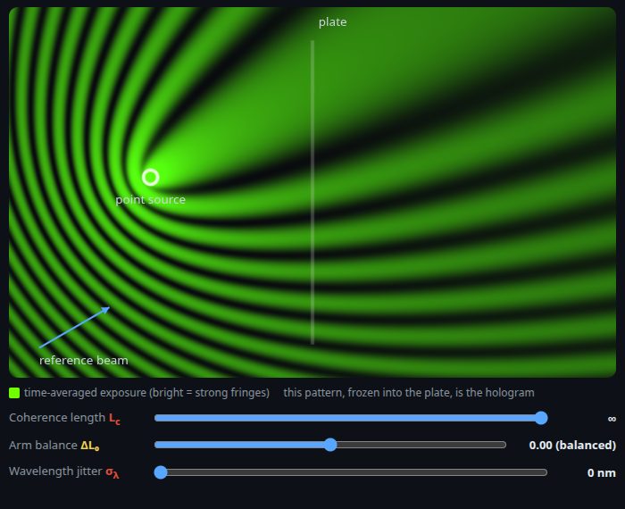
Fringe visibility between two arms with path difference \(\Delta L\) is V = exp(−(\(\Delta L\)/\(L_c\))²). As on a real table, the reference arm here includes a delay line: its path is extended by L₀ = d₁ + \(\Delta L_0\), where d₁ is the distance from source 1 to the plate center — so at \(\Delta L_0\) = 0 the two arms are balanced (ΔL = 0) at the plate center, standard practice before exposing a hologram. (With several sources the delay can only be matched to one; this demo balances to source 1.) Only the band where |\(d_{\mathrm{obj}}\)(y) − y sin \(\theta_R\) − L₀| < \(L_c\) records fringes, so shrinking \(L_c\) shrinks the effective aperture about the balance point: the reconstruction dims and blurs (resolution ∼ λ/aperture), exactly like a lens being stopped down. The \(\Delta L_0\) slider detunes the delay line and slides the recording band across (and off) the plate; and because the delay also advances the reference phase, the fringes crawl as you drag it.
Long \(L_c\) — fringes recorded across the whole aperture: bright, sharp reconstruction.
Short \(L_c\) — only the band where object and reference path lengths agree records fringes: smaller effective aperture, dim and blurred.
12b. Recording jitters and plate grain
A hologram is an exposure-time average: any noise that moves the fringes by ~\(\lambda/4\) during exposure erases them. For Gaussian jitter the fringe visibility between two arms picks up analytic factors:
Derivation
Every visibility factor is the same one-line average: for a Gaussian random phase φ with standard deviation \(\noi{\sigma_\phi}\),
so a fringe whose phase jitters by \(\noi{\sigma_\phi}\) during the exposure keeps visibility V = \(e^{-\noi{\sigma_\phi}^2/2}\). Each knob just supplies its own \(\noi{\sigma_\phi}\).
Wavelength jitter. A fringe between two arms with path difference \(\Delta L\) has phase φ = \(k\) \(\Delta L\), and a wavelength spread \(\sigma_\lambda\) maps to a wavenumber spread through the Jacobian \(|dk/d\lambda| = 2\pi/\lambda^2\) (from \(k = 2\pi/\lambda\)) — that is the \(\sigma_k\) in the first equation above. Matching its form against V = exp[−(\(\Delta L\)/\(L_c\))²] identifies \(L_c\) = √2/\(\sigma_k\).
Reference-angle jitter. The reference phase at plate height \(y\) is \(k\) \(y\) sin \(\theta_R\), so differentiating in \(\theta_R\), a small wobble δθ shifts it by δφ = \(k\) \(y\) cos \(\theta_R\) · δθ — the second equation above. Because δφ grows with |\(y\)|, fringes survive only near the plate center: an effective aperture.
Arm-path jitter. A path wobble \(\sigma_L\) shifts the phase directly, δφ = 2π\(\sigma_L\)/\(\lambda_R\), the same at every \(y\) — hence the uniform fade of the arm-path equation below, and the \(\lambda/4\) rule.
Wavelength jitter (laser linewidth — an LED is \(\sigma_\lambda\) ~ tens of nm) suppresses fringes wherever the object–reference path difference ΔL is large: it is literally the same physics as the coherence-length slider, expressed as a noise amplitude. Angle jitter (beam pointing, a vibrating mirror, an unstable table) moves the reference phase by \(k\)·\(y\)·cos\(\theta_R\)·δθ, which grows with distance from the plate center — fringes survive only within \(|y|\) < √2/(\(k\) cos\(\theta_R\) \(\sigma_\theta\)), so the effective aperture shrinks and the reconstruction blurs, exactly like stopping down a lens. This is why holography labs float their tables. In the full simulator, watch live-waves mode flicker when either jitter is up: that motion is what the time-average destroys. Object–object fringes are immune to reference-angle jitter (both arms share the source), but not to wavelength jitter.
Phase jitter — the reference arm's path length wobbles by \(\sigma_L\) (a mirror vibrating along the beam, air currents, thermal drift). The whole fringe comb slides sideways, so the contrast collapses uniformly over the plate:
This is the quarter-wave stability rule: a hologram tolerates path noise up to roughly \(\lambda\)/4, beyond which the contrast collapses quickly (the exponent grows quadratically). Unlike the other two jitters it has no spatial structure — nothing blurs, the whole image just fades. The slider is calibrated in units of \(\lambda\) and its readout shows V directly.
Steady table (\(\sigma_L\) = 0): the fringe comb holds still, full contrast.
Vibrating by \(\lambda/4\) (\(\sigma_L\) = \(\lambda/4\)): the comb blurs sideways — no detail lost, the whole image just fades.
Plate grain — additive emulsion noise \(\sigma_g\) on the developed transmittance t(y) (film grain, scattering centers). Grain does not move fringes, so it neither blurs nor fades the image; instead the random Δt diffracts light everywhere, burying the image under a diffuse haze — a noise floor rises in the retina strip while the spot stays sharp. Noise in the plate costs signal-to-noise ratio, not resolution. (The exposure view shows the noise-free average; the grain lives in the developed plate — see the plate strip in reconstruction mode.)
Add grain to the reconstruction in Figure 6 to see it. The recording jitter sliders \(\sigma_\theta\), \(\sigma_L\), \(\sigma_g\) are hidden in the figures but all live in the full simulator.
No grain — the image point is sharp against a dark field.
Grain (\(\sigma_g\) > 0) — same sharp point, now sitting in a diffuse speckle haze: lost signal-to-noise, not resolution.
12c. Replay-side noise
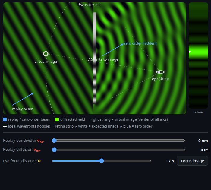
Replay-side noise — viewing with an imperfect source instead of recording with one. The retina is a time average, so a broadband source (\(\sigma_{\lambda P}\) > 0, an LED instead of a laser) or a diffuse one (\(\sigma_{\theta P}\) > 0, frosted glass, an extended lamp) just averages many detuned reconstructions incoherently. Each sample lands where the paraxial formulas above put it, so the spot smears over the sampled spread — the translucent white band in the retina strip marks exactly that predicted extent. Nothing about the plate changed: this is why a display hologram looks sharp under a laser pointer and rainbow-smeared under a white lamp. (The field view keeps showing the coherent reconstruction at the central replay values — an incoherent average has no single field to draw.)
Monochromatic replay — every ray images to the same place: one sharp point.
Broadband replay (\(\sigma_{\lambda P}\) > 0) — each colour focuses at a slightly different spot (μ differs), so the point drags out into a spectrum.
13. From the 2D slice to a real hologram
Everything on screen is one horizontal slice through the setup: the plate is a line, the point sources emit cylindrical waves, and the reference is a plane wave tilted within the plane. That slice is quantitatively honest — the grating equation, the wavelength dispersion, the three orders and their evanescence, coherence, aperture and resolution, the twin image, and the accommodation of the eye are all exactly the in-plane physics of the full problem. If the slice makes sense, the physics makes sense.
What you see — a horizontal cut. Each wavefront is a circle (a cylinder edge-on) and each fringe is a line.
The real plate — that same fringe set is a full 2-D ring pattern (a Fresnel zone plate), and each wavefront is a sphere. The dashed line is exactly the cut shown at left.
A real hologram is that slice swept into the third dimension, which adds what a 2D cut structurally can’t show:
• The fringe pattern is a 2D surface. A single point records a full circular/elliptical Fresnel zone plate on the (x, y) plate, not a 1D set of fringes. The line of fringes here is one horizontal cut across those rings (see the 2D→3D figure just above).
• Vertical parallax. The reconstructed wave is a true spherical wave, so the image shifts as you move your head up/down as well as left/right — you can look around foreground objects. White-light “rainbow” display holograms deliberately throw away vertical parallax (via a slit) so they can be lit by an extended source without the dispersion smearing the image.
• Orders and pupils become 2D. The 0/±1/conjugate orders separate into directions in 3-space (cones, not a fan), and the eye integrates over a 2D pupil rather than a slit — so real resolution goes as λ/D with D the pupil diameter in both axes.
• Volume effects. A thick emulsion adds Bragg selection along the plate’s depth, which is what makes a Denisyuk reflection hologram pick its own colour out of white light and suppresses the conjugate entirely — genuinely 3D behaviour with no 2D analogue.
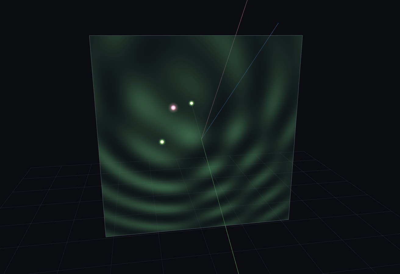
So: read this slice for the mechanism, then picture every fringe line as a ring and every fan of rays as a cone to get the real object.
14. Holographic interferometry
Everything so far has used holography to reconstruct a scene. Its most useful measurement application turns that around: rather than admire the image, compare two recordings of the same object and read the tiny difference between them. By how much did a turbine blade bow under load? Which parts of a loudspeaker cone or a violin plate move at a given driving frequency, and how far? Holographic interferometry answers questions like these over the whole surface at once, without touching the object, to a fraction of a wavelength — tens of nanometres.
Ordinary interferometry already reaches that precision, but only by comparing a wavefront against a smooth reference surface, which confines it to polished optics. Holography removes the restriction. Because the plate stores the actual wavefront a surface returned — rough, matte, whatever its shape — the object can act as its own reference: compare the wave it sends now against a recording of the wave it sent before, and any change in the surface appears directly. That is the whole idea, and it works on ordinary machined and cast parts, not just mirrors.
Concretely: record the wavefront in two states of the object — before and after it is loaded, heated, or set vibrating. Wherever the two states have drifted apart by half a wave the waves cancel, so the reconstruction is crossed by dark fringes, and each fringe is a contour line of the surface displacement — successive fringes a fraction of a micron apart in movement. Read the fringes and you have measured the deformation everywhere at once.
The idea is one comparison. Two object waves \(O_1\) and \(O_2\) that differ only by a small surface displacement \(\geo{\mathbf{d}}\) differ in phase by the extra path the light travels to the moved surface and back:
where the sensitivity vector \(\geo{\mathbf{S}}\) is the difference of the unit vectors toward the observer and toward the source — the direction, and amount, of displacement the setup can see. Its length runs from 0 (a motion the geometry is blind to) up to 2 (straight-on illumination and viewing, the most sensitive case, where one fringe means just \(\rec{\lambda}/2\) of movement). Where \(\Delta\varphi\) is a multiple of \(2\pi\) the two waves add; where it is an odd multiple of \(\pi\) they cancel. Each method below is a way to make one plate hold both waves at once and let them interfere.
Double-exposure: two states on one plate
The simplest method exposes a single plate twice before developing — once with the object at rest, once after it has moved. The plate sums the two intensity patterns, so it stores both fringe systems; replay reconstructs \(O_1\) and \(O_2\) together and they interfere, laying a cosine fringe pattern over the reconstructed image:
Derivation
The two exposures deposit \(I_1 = |O_1 + R|^2\) and \(I_2 = |O_2 + R|^2\), and the developed transmittance is their sum. Its image-carrying part is the cross term
a single grating written by the combined object wave \(O_1 + O_2\). Replaying with \(R\) sends the \(\ord{m}=+1\) order into \(E \propto O_1 + O_2\), so the reconstructed intensity is \(|O_1 + O_2|^2\). With \(|O_1|\approx|O_2|\approx|O|\) and a phase difference \(\Delta\varphi = \arg O_1 - \arg O_2\) this is \(2|O|^2(1 + \cos\Delta\varphi)\) — bright where the two states agree, dark where they are half a wave apart.
In the 2-D slice the “object” is a point source, so a “displacement” is a shift of that source. Figure 7 records it twice and shows the reconstructed intensity: at zero shift the image is clean; raise the object displacement and dark interferometric fringes fill the field, one more appearing for every extra half-wave of path difference across it. Count the fringes and you have read the displacement. Undo the shift and the fringes vanish; push it further and more crowd in.
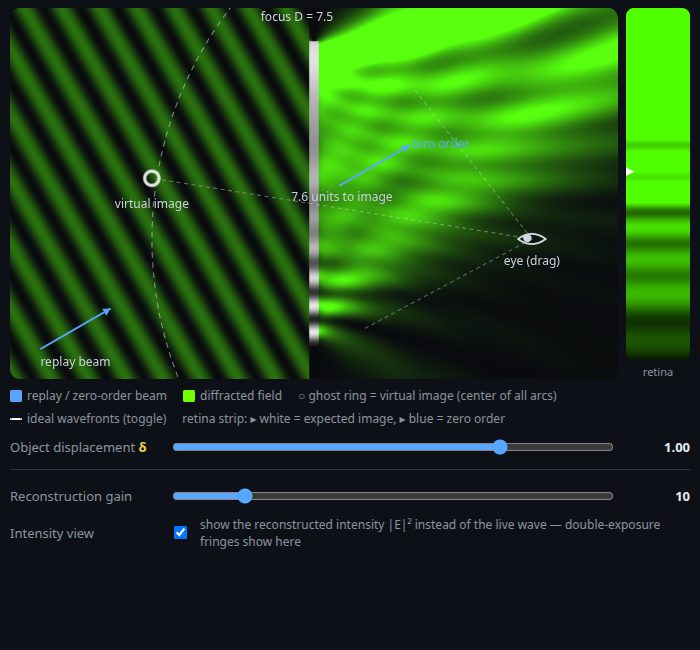
Because \(\Delta\varphi\) depends on \(\geo{\mathbf{S}}\cdot\geo{\mathbf{d}}\), a fringe is a contour of constant displacement along the sensitivity vector: with straight-on viewing the fringes map out-of-plane motion in steps of \(\rec{\lambda}/2\); tilt the geometry and the same fringes weigh a different component of the motion. On a real 3-D object those contours lie on the surface like a topographic map of how it moved.
A point that moves by d lengthens the path source → point → eye by S·d, where the sensitivity vector S bisects the illumination and viewing directions. One fringe marks every half-wave of that change, so the fringes are contours of the displacement along S.
Real-time: watch the fringes move
Develop the hologram and leave it exactly where it was recorded. Now look at the live object through the plate: it reconstructs the object wave from the recorded state, \(O_{\text{rec}}\), and that interferes with the light coming from the object now, \(O_{\text{live}}(t)\):
As the object deforms the fringes crawl across it in real time, one sweeping past for every half-wave of motion — so you watch the deformation develop rather than freezing a single before/after pair. When the object returns to its recorded shape \(\Delta\varphi \to 0\) and the field goes uniformly dark: the live and reconstructed waves match everywhere. The catch is contrast — the reconstructed wave is dimmer than a fresh exposure, so real-time fringes are fainter than double-exposure ones.
Looking at the live object through its developed hologram: the recorded wavefront and the present one interfere, and the fringes crawl as the object deforms — going dark everywhere the moment it returns to its recorded shape.
Time-average: mapping a vibration
Aim the same setup at something vibrating and expose for many cycles. The plate records the time-average of the object wave over the vibration. A patch oscillating with amplitude \(a\) sweeps back and forth through a range of phase, and averaging that motion weights its reconstructed brightness by a Bessel function:
Where the surface barely moves, \(a \to 0\) and \(J_0^2 \to 1\): the nodes stay brightest. The antinodes are crossed by the dark zeros of \(J_0\) (at argument 2.40, 5.52, 8.65, …), so a single exposure maps the vibration’s mode shape and amplitude at once — holography’s answer to Chladni’s sand figures. Unlike the cosine fringes of the other two methods these fade with each order, because \(J_0\) decays.
Time-average holography of a vibrating cantilever: the still node at the clamp stays brightest, and the dark J0 fringes crowd toward the swinging tip — a contour map of the mode shape and its amplitude.
15. How the simulator propagates the replayed field
Every point to the right of the plate in reconstruction mode is one integral over the plate line: the exit field \(t(\geo{y})\cdot e^{i\rep{k_P}\,\geo{y}\sin\rep{\theta_P}}\), propagated to the field point P by the two-dimensional Rayleigh–Sommerfeld integral of the first kind:
Derivation
In 2D the outgoing free-space Green’s function of the Helmholtz equation is G = (i/4)·\(H_0^{(1)}\)(\(k_P\) r) — a Hankel function takes the place of the familiar \(e^{ikr}\)/r. The Rayleigh–Sommerfeld construction of the first kind (the field on the plate line weighted by the normal derivative of G) gives
where \(d\) = |P − (0, \(y\))| and the (x/\(d\)) obliquity factor comes from the normal derivative ∂/∂x of \(H_0^{(1)}\). For \(k_P\) \(d\) ≫ 1 the Hankel function has the asymptotic form \(H_1^{(1)}\)(z) ≈ √(2/πz)·\(e^{i(z - 3\pi/4)}\); substituting it recovers the integral displayed above, which is exactly what the shader evaluates with a 512-point midpoint rule. The constant phase \(e^{-i\pi/4}\) is dropped, since only relative phase and intensity are displayed, and the 1/√\(d\) amplitude falloff is the 2D counterpart of the 3D 1/r. Writing t = t̄ + Δt splits this integral into the attenuated replay beam and the image-carrying wave, which is all the “Hide zero-order beam” toggle does: it drops the t̄ term.
16. Numbers and conventions
Scene units are arbitrary; the plate half-height defaults to 3. Wavelength maps to scene units at 1 nm = 0.0012 units (so 532 nm → 0.64 units) — hugely exaggerated so fringes are visible, the same trade-off the 3Blue1Brown video makes. Reference amplitude \(A_{\mathrm{ref}}\) = 0.7; object waves fall off as 1/√d. Thin amplitude-hologram efficiency peaks at 1/16 = 6.25% per first order. The plate transmittance is sampled at 2048 points and the reconstruction integral (Rayleigh–Sommerfeld, first kind) at 512 points; the eye pupil is 6 units wide and its retina is a 48-sample focus scan; replay-noise averaging uses 13 quasi-Gaussian samples. The wave animation runs at a fixed phase speed.
References
- D. Gabor. A new microscopic principle. Nature 161, 777–778 (1948). doi:10.1038/161777a0
- P. Hariharan. Optical Holography: Principles, Techniques, and Applications, 2nd ed. Cambridge University Press (1996).
- E. N. Leith and J. Upatnieks. Reconstructed wavefronts and communication theory. J. Opt. Soc. Am. 52, 1123–1130 (1962). doi:10.1364/JOSA.52.001123
- S. A. Benton. Hologram reconstructions with extended incoherent sources. J. Opt. Soc. Am. 59, 1545 (1969) — the rainbow (white-light transmission) hologram.
- Yu. N. Denisyuk. Photographic reconstruction of the optical properties of an object in its own scattered radiation field. Sov. Phys. Dokl. 7, 543 (1962) — the reflection (volume) hologram.
- J. W. Goodman. Introduction to Fourier Optics, 3rd ed. Roberts & Company (2005) — the Rayleigh–Sommerfeld diffraction integrals.
- G. Sanderson (3Blue1Brown). Holograms. Source scenes at 3b1b/videos/_2024/holograms (2024).
- C. M. Vest. Holographic Interferometry. Wiley (1979) — the standard reference on the method.
- R. L. Powell and K. A. Stetson. Interferometric vibration analysis by wavefront reconstruction. J. Opt. Soc. Am. 55, 1593–1598 (1965). doi:10.1364/JOSA.55.001593 — time-average holography.