The toy session
Every concept in this tutorial is introduced on a toy order-book
session you can verify with mental arithmetic before it is shown on
real data: 24 events, 12 orders, 5 trades, one synthetic minute, prices
98–103 around a mid of 100, sizes 1 to 3. It ships in the package —
toy_events() and toy_trades() return ordinary DataFrames in exactly
the layout every real loader produces, so everything you do with them
works unchanged on a 300,000-event capture.
The orders, and what happens to each:
| Actor | Order | Outcome | Classified as |
|---|---|---|---|
| Alice | bid 2 @ 99 (t=0) | filled fully by Sam's sweep (t=56) | resting-limit |
| Bob | ask 3 @ 101 (t=2) | filled by Frank (1) then Hana (2) | resting-limit |
| Chen | bid 1 @ 98 (t=5) | still in the book at the end | resting-limit |
| Ivy | bid 2 @ 99 (t=6) | queued behind Alice; only 1 fills (t=57) | resting-limit |
| Dana | bid 3 @ 98 (t=8) | cancelled (t=40) | flashed-limit |
| Erin | ask 2 @ 102 (t=12) | survives | resting-limit |
| Frank | market buy 1 (t=20) | crosses the spread, fills against Bob | market |
| Gus | ask 2 @ 103 (t=35) | survives | resting-limit |
| Eve | bid 1 @ 100 (t=45.0) | pulled after 800 ms — a flash | flashed-limit |
| Hana | bid 3 @ 101 (t=48) | takes 2 from Bob, rests 1, later hit | market-limit |
| Iris | market sell 1 (t=52) | hits Hana's resting order | market |
| Sam | market sell 3 (t=56) | sweeps the 99 queue: Alice fully, Ivy half | market |
%matplotlib inline
from ob_analytics import toy_events, toy_trades

events = toy_events()
trades = toy_trades()
events.head(6)[["event_id", "actor", "action", "direction", "price", "volume", "fill"]]
| event_id | actor | action | direction | price | volume | fill | |
|---|---|---|---|---|---|---|---|
| 0 | 1 | Alice | created | bid | 99 | 2 | 0 |
| 1 | 2 | Bob | created | ask | 101 | 3 | 0 |
| 2 | 3 | Chen | created | bid | 98 | 1 | 0 |
| 3 | 4 | Ivy | created | bid | 99 | 2 | 0 |
| 4 | 5 | Dana | created | bid | 98 | 3 | 0 |
| 5 | 6 | Erin | created | ask | 102 | 2 | 0 |
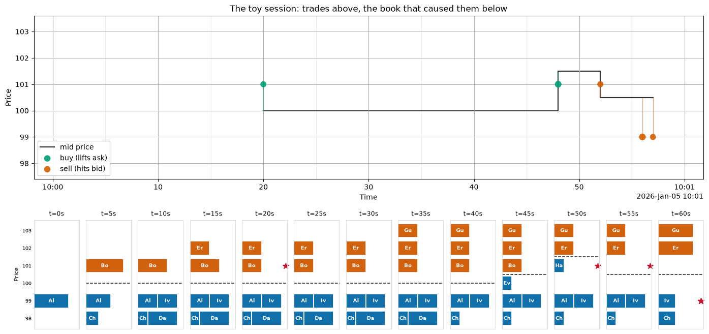
The stream replayed: the trade tape on top shows only the five executions — the effects. The strip below shows the causes: the full book every five seconds, each order labeled, queued in arrival order (first arrival nearest the axis). Watch Ivy line up behind Alice at 99 (t=10), Dana vanish at t=40, Eve's flash exist for exactly one frame (t=45) — moving the mid without a single trade — and Sam's sweep leave only half of Ivy standing (t=60).
import matplotlib.pyplot as plt
import pandas as pd
from _docs_theme import DOCS_THEME, plot_book_keyframes

from ob_analytics.analytics import set_order_types
from ob_analytics.depth import depth_metrics, get_spread, price_level_volume
from ob_analytics.visualization import plot, prepare

classified = set_order_types(events, trades)
spread = get_spread(depth_metrics(price_level_volume(classified)))

fig = plt.figure(figsize=(17, 8))
gs = fig.add_gridspec(2, 13, height_ratios=[1.5, 1.0], hspace=0.3, wspace=0.15)
ax_tape = fig.add_subplot(gs[0, :])
plot(
    "trade_tape",
    level="L2",
    ax=ax_tape,
    theme=DOCS_THEME,
    **prepare.trades(trades, spread=spread),
)
# The face steps the mid natively; darken it for the tutorial and give it
# a legend entry so the reference line is unmissable next to the gridlines.
for i, line in enumerate(ax_tape.get_lines()):
    line.set_color("#333333")
    line.set_linewidth(1.6)
    line.set_alpha(1.0)
    if i == 0:
        line.set_label("mid price")
t0 = events["timestamp"].iloc[0]
for k in range(0, 61, 5):
    ax_tape.axvline(t0 + pd.Timedelta(seconds=k), color="#e3e3e3", lw=0.5, zorder=0)
# Share the keyframes' price frame so the panels correspond level for level
# (the tape would otherwise autoscale to the traded range and hide 102/103).
ax_tape.set_ylim(events["price"].min() - 0.6, events["price"].max() + 0.6)
ax_tape.set_yticks(sorted(events["price"].unique()))
ax_tape.margins(x=0.03)
ax_tape.legend(loc="lower left", framealpha=0.9)
ax_tape.set_title("The toy session: trades above, the book that caused them below")

key_axes = [fig.add_subplot(gs[1, i]) for i in range(13)]
for axk in key_axes[1:]:
    axk.sharey(key_axes[0])
plot_book_keyframes(classified, trades, ax_row=key_axes)
for axk in key_axes[1:]:
    axk.tick_params(labelleft=False)
Twelve orders, four classes. set_order_types assigns each order its
type from the raw events — with these twelve, every classification is
checkable by eye against the table above:
actor
Dana     flashed-limit
Eve      flashed-limit
Alice    resting-limit
Bob      resting-limit
Chen     resting-limit
Erin     resting-limit
Gus      resting-limit
Ivy      resting-limit
Hana      market-limit
Frank           market
Iris            market
Sam             market
Name: type, dtype: category
Categories (6, str): ['unknown' < 'pre-existing' < 'flashed-limit' < 'resting-limit' < 'market-limit' < 'market']
Step through it yourself
The keyframes above show the book every five seconds. The replay below
shows it every second, and you control it: drag the slider, or press a
play button (Play 1× is real time, so the whole minute takes a
minute). The ladder on the left is the L3 book, one segment per order,
queued in arrival order. The panel on the right is the trade tape, with
a line at the time on screen. Click a trade to jump to the book just
before it, with the price level it took marked.
replay = prepare.book_replay(
    events=classified, trades=trades, per_order=True, price_levels=3
)
plot("book_replay", level="L3", backend="plotly", **replay)
Things to look for: Eve's bid at 100 exists for exactly one frame (t=45); Hana's order at 101 takes Bob's last two lots and rests one lot for four seconds (t=48–51); and after Sam's sweep (t=56–57), only half of Ivy is left at 99.
Change the script
The toy session is a script of twelve orders, and you can rewrite it.
toy_orders() returns the script as a dictionary of ToyOrders keyed
by actor. Add an order, remove one, or change when an order is
cancelled, then match_toy_orders matches the new script by
price–time priority and returns its events and trades, in the same
layout as toy_events() and toy_trades(). A market order is a limit
order priced through the touch, as Frank's bid at 101 is.
Here a new trader, Jo, posts a bid of 1 lot at 100 at t=10, and Dana never places her order:
from ob_analytics import ToyOrder, match_toy_orders, toy_orders

orders = toy_orders()
orders["Jo"] = ToyOrder(at=10, direction="bid", price=100, volume=1)
del orders["Dana"]
edited_events, edited_trades = match_toy_orders(orders)
edited_trades[["timestamp", "price", "volume", "maker_actor", "taker_actor"]]
| timestamp | price | volume | maker_actor | taker_actor | |
|---|---|---|---|---|---|
| 0 | 2026-01-05 10:00:20+00:00 | 101 | 1 | Bob | Frank |
| 1 | 2026-01-05 10:00:48+00:00 | 101 | 2 | Bob | Hana |
| 2 | 2026-01-05 10:00:52+00:00 | 101 | 1 | Hana | Iris |
| 3 | 2026-01-05 10:00:56+00:00 | 100 | 1 | Jo | Sam |
| 4 | 2026-01-05 10:00:56+00:00 | 99 | 2 | Alice | Sam |
Jo's bid is now the best bid from t=10, so Sam's sell at t=56 fills Jo first, at 100, and only then Alice at 99. Ivy, who was half-filled in the original session, is not reached at all. The same two lines that drew the first replay draw the edited one:
edited = set_order_types(edited_events, edited_trades)
replay = prepare.book_replay(
    events=edited, trades=edited_trades, per_order=True, price_levels=3
)
plot("book_replay", level="L3", backend="plotly", **replay)
One difference from the hand-written session: match_toy_orders fills
all of Sam's sell at t=56, as a matching engine would, where the
hand-written session prints Ivy's fill a second later so the keyframes
can show the book between the two fills. Every other event is the
same: match_toy_orders(toy_orders()) rebuilds the toy session.
Chapters 2, 4 and 6 end with exercises. In chapters 2 and 4 you change this script, predict what happens, and check your prediction against the library; each exercise has a solution you can open after you try it.
The same mechanics at full scale
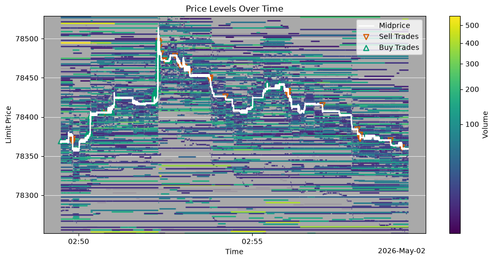
Everything above transfers unchanged to real data. The bundled sample is a ~30-minute Bitstamp BTC/USD capture — ~314,000 events instead of 24, thousands of price levels instead of five. The depth heatmap below (zoomed to the capture's busiest ten minutes) is nothing but the keyframe strip compressed into pixels: one column per instant, one row per price, brightness = resting volume.
from _docs_theme import plot_sample_heatmap

from ob_analytics import Pipeline, sample_csv_path
from ob_analytics.visualization import display_result

result = Pipeline().run(sample_csv_path())
# Canonical prices are integer ticks (issue #155); show quote currency.
result = display_result(result)
fig = plot_sample_heatmap(result, col_bias=0.4)
Next: chapter 1 starts from zero — what a price actually is, what an exchange does, and why the number on a brokerage app was an order book all along.