From a price to an order book
This chapter assumes no finance knowledge — only things you already know: buying, selling, and a number on a screen. By the end, that number will be a live data structure you can query, replay, and plot.
What a price actually is
Look up bitcoin, or a share of Apple, and you get one number. It feels like a fact about the world, the way a temperature is.
It isn't. A price is only ever the last deal two people agreed to. Think of a market stall: the seller asks 105, you offer 95, you settle at 100 — and now the melon "costs" 100, until the next haggle ends differently. Between deals there is no price; there are only people willing to buy at some number and people willing to sell at another.
What an exchange actually does
Haggling works for one melon. It does not work for thousands of strangers trading the same thing every second — nobody can bargain face-to-face with a crowd. An exchange (a bourse) solves this with two moves:
- Everyone writes down a firm, standing offer: "I'll buy 2 at 99 or less", "I'll sell 3 at 101 or more". No haggling, no take-backs while it stands.
- A neutral matching engine pairs compatible offers by fixed, public rules.
This arrangement is called a continuous double auction — "double" because both buyers and sellers post offers, "continuous" because it runs all day, not at a scheduled hour. And the public list of standing offers, sorted by price, is the order book. The rest of this tutorial is about reading it.
flowchart LR
    T1[Buyers] -- "bid: buy 2 @ 99" --> ME{{matching engine}}
    T2[Sellers] -- "ask: sell 3 @ 101" --> ME
    ME -- "compatible? trade!" --> TAPE[trade tape]
    ME -- "not yet? it waits" --> BOOK[(order book)]
If you've used eBay, you already know both modes: buy-it-now is taking a standing offer; make-an-offer is posting one and waiting.
Level 1: the number you already knew
So what does a brokerage app actually show? Three numbers, usually collapsed into one:
%matplotlib inline
from _docs_theme import DOCS_THEME

from ob_analytics.visualization import plot

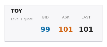
fig = plot("l1_ticker", bid=99, ask=101, last=None, symbol="TOY", theme=DOCS_THEME)
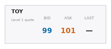
- the best bid — the highest standing buy offer (someone will pay you 99 right now),
- the best ask — the lowest standing sell offer (someone will sell to you at 101 right now),
- the last trade — the most recent deal (none yet, hence the dash).
This triplet is called Level 1 (L1) market data, and it's what tickers, apps, and headlines mean by "the price". Notice there is no single price in it: buying costs you 101, selling gets you 99, and the quoted "price" is usually just the midpoint or the last print.
This is the theme of the whole tutorial: each finer level of market data simply summarizes less. L1 keeps the top of the book; the book keeps everything.
Two orders: the book
Now build that quote card from orders. We'll use the package's toy session — a hand-written minute of trading small enough to check by mental arithmetic. At t=0, Alice posts a bid: buy 2 at 99 or better. Two seconds later, Bob posts an ask: sell 3 at 101 or better.
import pandas as pd

from ob_analytics import toy_events, toy_trades
from ob_analytics.analytics import set_order_types

events = set_order_types(toy_events(), toy_trades())  # adds a `type`
# column we'll need soon — ignore it until the classification section.
t0 = events["timestamp"].iloc[0]

events.head(2)[["event_id", "actor", "action", "direction", "price", "volume"]]
| event_id | actor | action | direction | price | volume | |
|---|---|---|---|---|---|---|
| 0 | 1 | Alice | created | bid | 99 | 2 |
| 1 | 2 | Bob | created | ask | 101 | 3 |
order_book() reconstructs the standing offers at any instant.
Here is the book three seconds in, drawn as a ladder — price on the
vertical axis, size on the horizontal, bids in blue below, asks in
orange above:
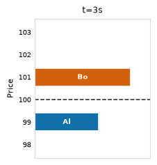
Read everything off the picture: best bid 99, best ask 101. The gap between them — 101 − 99 = 2 — is the spread: the cost of being impatient, since buying immediately and selling immediately loses you the spread. The dashed line at (99 + 101) / 2 = 100 is the mid price, the book's reference "price" even though nobody is offering to trade there. Our L1 card above was exactly this picture's top row — nothing more.
A queue forms
More people arrive. Chen bids 1 at 98, Ivy bids 2 at 99 — the same price as Alice — Dana bids 3 at 98, and Erin asks 2 at 102:
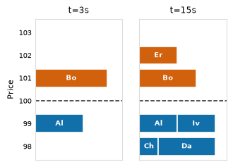
At 99 there are now two orders. Who gets filled first when a seller finally arrives? The matching engine's rule is price–time priority: better prices trade first, and at the same price, whoever arrived first trades first. In the ladder, each order is its own segment, stacked in arrival order from the axis outward — Alice (t=0) sits ahead of Ivy (t=6) at 99, Chen (t=5) ahead of Dana (t=8) at 98. The queue is an ordered list, and its order decides who trades first; we return to it at the end of the minute.
A trade
At t=20, Frank wants to buy 1 now. He doesn't post an offer and wait — he prices his order to cross the spread (a market order), and the engine matches him with the best ask: Bob.
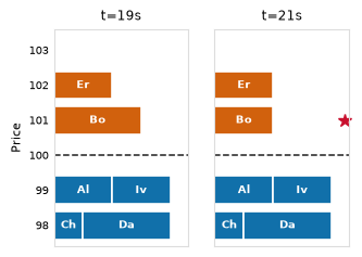
Compare the frames: Bob's bar shrank from 3 to 2 — he sold 1 to Frank at 101 (the star). The trade tape records the deal, and the roles have names: Bob, whose standing offer was consumed, is the maker (he made liquidity by resting in the book); Frank, who crossed to take it, is the taker. Every trade has exactly one of each:
trades = toy_trades()
trades.head(1)[
    ["timestamp", "price", "volume", "direction", "maker_actor", "taker_actor"]
]
| timestamp | price | volume | direction | maker_actor | taker_actor | |
|---|---|---|---|---|---|---|
| 0 | 2026-01-05 10:00:20+00:00 | 101 | 1 | buy | Bob | Frank |
And the L1 card updates: LAST is finally a number.
A cancellation, and a flash
Standing offers are commitments, but you can cancel them. At t=40 Dana cancels her entire bid at 98. And at t=45.0 Eve posts a bid at 100 — inside the spread, briefly narrowing it — then cancels it 800 milliseconds later:
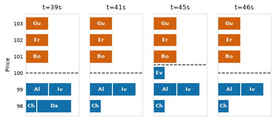
Dana's departure (t=41 vs t=39) removed liquidity without a single trade printing. Eve's flashed order existed for under a second — but look at the dashed mid line at t=45: her bid at 100 dragged the mid up to 100.5. The market's "price" moved and no one traded. On a trades-only data feed, neither event exists.
These behaviours are so characteristic that the package classifies every order's lifetime automatically:
actor
Dana     flashed-limit
Eve      flashed-limit
Alice    resting-limit
Bob      resting-limit
Chen     resting-limit
Erin     resting-limit
Gus      resting-limit
Ivy      resting-limit
Hana      market-limit
Frank           market
Iris            market
Sam             market
Name: type, dtype: category
Categories (6, str): ['unknown' < 'pre-existing' < 'flashed-limit' < 'resting-limit' < 'market-limit' < 'market']
The four classes: resting-limit (posted, waited — filled or still standing), market (crossed immediately: Frank, Iris, Sam), market-limit (crossed, then the remainder rested: Hana — chapter 2 tells her story), and flashed-limit (posted and cancelled unfilled: Dana and Eve).
Pitfall: 'flashed' means unfilled, not fast
The classifier labels any order that was created and fully
cancelled without trading as flashed-limit — Dana rested for 32
seconds and gets the same label as Eve's 800 ms.
If your analysis needs true sub-second flashes (quote-stuffing
detection, for instance), filter on lifetime as well as type.
Adding time: the whole minute at once
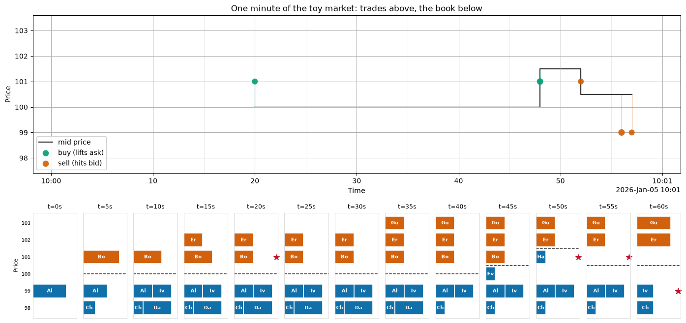
You have now seen every mechanism the book has: post, queue, trade, cancel, flash. Here is the full minute — the tape of effects above, and below it the book (the causes) every five seconds. Watch the 99 queue: Sam's market sell of 3 at t=56 fills Alice completely and Ivy only half, purely because Alice arrived six seconds earlier. That is the consequence of price–time priority.
import matplotlib.pyplot as plt
from _docs_theme import DOCS_THEME

from ob_analytics.depth import depth_metrics, get_spread, price_level_volume
from ob_analytics.visualization import plot, prepare

spread = get_spread(depth_metrics(price_level_volume(events)))

fig = plt.figure(figsize=(17, 8))
gs = fig.add_gridspec(2, 13, height_ratios=[1.5, 1.0], hspace=0.3, wspace=0.15)
ax_tape = fig.add_subplot(gs[0, :])
plot(
    "trade_tape",
    level="L2",
    ax=ax_tape,
    theme=DOCS_THEME,
    **prepare.trades(trades, spread=spread),
)
for i, line in enumerate(ax_tape.get_lines()):
    line.set_color("#333333")
    line.set_linewidth(1.6)
    line.set_alpha(1.0)
    if i == 0:
        line.set_label("mid price")
for k in range(0, 61, 5):
    ax_tape.axvline(t0 + pd.Timedelta(seconds=k), color="#e3e3e3", lw=0.5, zorder=0)
ax_tape.set_ylim(events["price"].min() - 0.6, events["price"].max() + 0.6)
ax_tape.set_yticks(sorted(events["price"].unique()))
ax_tape.margins(x=0.03)
ax_tape.legend(loc="lower left", framealpha=0.9)
ax_tape.set_title("One minute of the toy market: trades above, the book below")

key_axes = [fig.add_subplot(gs[1, i]) for i in range(13)]
for axk in key_axes[1:]:
    axk.sharey(key_axes[0])
plot_book_keyframes(events, trades, ax_row=key_axes)
for axk in key_axes[1:]:
    axk.tick_params(labelleft=False)
The same mechanics at full scale
Twenty-four events fit in thirteen hand-drawn frames. A real market does hundreds of events per second — so we compress: one column per instant, one row per price, and brightness for resting volume. That is all a depth heatmap is: the keyframe strip above, squeezed into pixels. Below, the busiest ten minutes of the bundled ~30-minute Bitstamp BTC/USD capture — the mechanics you just watched one at a time, hundreds of times per second:
from _docs_theme import plot_sample_heatmap

from ob_analytics import Pipeline, sample_csv_path
from ob_analytics.visualization import display_result

result = Pipeline().run(sample_csv_path())
# Canonical prices are integer ticks (issue #155); show quote currency.
result = display_result(result)
fig = plot_sample_heatmap(result, col_bias=0.4)
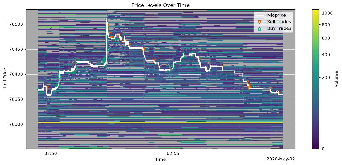
Bright bands are heavy standing offers (the crowd's version of Dana's 3-lot); the dark band through the middle is the spread around the mid — the same dashed line as in the toy frames.
Next: L1 → L2 → L3 — three resolutions of the same market, and what each one can and cannot answer.
Vocabulary introduced here — bourse, matching engine, continuous double auction, Level 1 / best bid / best ask / last, spread, mid price, price–time priority, maker / taker, market order — lives in the Glossary.