L1 → L2 → L3: three resolutions of the same market
Chapter 1 ended with an idea: each finer level of market data summarizes less. This chapter makes it precise. Market data comes in three standard resolutions, and they nest like map zoom levels — city, street, building. Same territory, three levels of detail, and each level is a lossy summary of the next: you can always compute L1 from L2, and L2 from L3, but never the reverse.
One instant, three renderings
Here is the toy session's book at t=30s, drawn at all three resolutions at once:
%matplotlib inline
import matplotlib.pyplot as plt
import pandas as pd

from ob_analytics import toy_events, toy_trades
from ob_analytics.analytics import order_book, set_order_types
from ob_analytics.visualization import plot, prepare

events = set_order_types(toy_events(), toy_trades())
t30 = events["timestamp"].iloc[0] + pd.Timedelta(seconds=30)
snap = order_book(events, tp=t30)

fig, (ax1, ax2, ax3) = plt.subplots(1, 3, figsize=(15, 4.4))
plot("l1_ticker", ax=ax1, bid=99, ask=101, last=101, symbol="TOY")
ax1.set_title("L1 — the quote", fontsize=10)
plot("book_snapshot", level="L2", ax=ax2, **prepare.book_snapshot(snap))
ax2.set_title("L2 — market by price", fontsize=10)
plot("book_snapshot", level="L3", ax=ax3, **prepare.book_snapshot(snap, per_order=True))
ax3.set_title("L3 — market by order", fontsize=10)
fig.tight_layout()
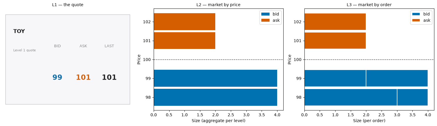
Read it left to right, adding detail as you go:
- L1 is the quote: best bid 99, best ask 101, last 101. Three numbers, nothing else.
- L2 (market by price) unfolds the quote into the full ladder — every price level with its total size: 4 at 99, 4 at 98, not just the best. L1 was this picture's top row.
- L3 (market by order) splits each bar into its owners: at 99 those 4 units are two bids (Alice's 2 and Ivy's 2), at 98 two more. Identity and queue position appear.
Now run it backwards: each panel is a lossy summary of the one to its right. Summing L3's segments gives you L2 exactly; keeping L2's top row gives you L1 exactly. The reverse is impossible — who owns the 4 at 99, and who is first in line, cannot be recovered from the bar's length.
Same L2, different markets
How much does the L3 → L2 summary destroy? Here are two ask books that are identical at L2 — four units offered at 101 — drawn at both resolutions:
whale = {
    "timestamp": t30,
    "bids": pd.DataFrame({"id": [1], "price": [99.0], "volume": [4.0]}).iloc[:0],
    "asks": pd.DataFrame({"id": [10], "price": [101.0], "volume": [4.0]}),
}
crowd = {
    "timestamp": t30,
    "bids": whale["bids"],
    "asks": pd.DataFrame(
        {"id": [21, 22, 23, 24], "price": [101.0] * 4, "volume": [1.0] * 4}
    ),
}

fig, axes = plt.subplots(2, 2, figsize=(10, 6), sharex=True, sharey=True)
for col, (name, book) in enumerate([("one whale", whale), ("a crowd", crowd)]):
    plot("book_snapshot", level="L2", ax=axes[0][col], **prepare.book_snapshot(book))
    axes[0][col].set_title(f"L2 — {name}", fontsize=10)
    plot(
        "book_snapshot",
        level="L3",
        ax=axes[1][col],
        **prepare.book_snapshot(book, per_order=True),
    )
    axes[1][col].set_title(f"L3 — {name}", fontsize=10)
for ax in axes.ravel():
    ax.set_ylim(100.4, 101.6)
    ax.legend().remove()
fig.tight_layout()
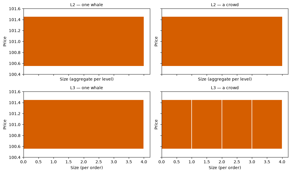
The top row is indistinguishable. The bottom row is two different markets: a single 4-lot (one order, which can be cancelled all at once) versus four independent 1-lots. If you trade against it, the difference matters: the whale cancelling removes all the liquidity at once; the crowd thins out one order at a time. L2 cannot tell you which market you're in. That is the information L3 buys you.
Why L3 exists: the queue
Chapter 1 showed the 99-bid queue as stacked bars. The package's queue engine turns that into a quantitative face: each resting order's FIFO rank at the touch over time — rank 1 is the front of the line — coloured by its outcome. Every trajectory below is labeled with its owner, and the book ladders underneath show the decisive instants:
from _docs_theme import plot_queue_story

fig = plot_queue_story(events, toy_trades(), at_s=[6, 45, 56, 57])
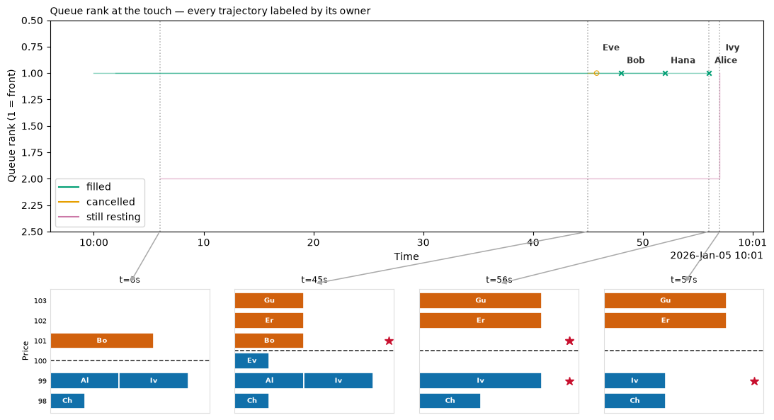
Now the walk is literal:
- Ivy (pink) is the clearest case: she joins the 99 queue at t=6 at
rank 2 — the ladder below shows her stacked behind Alice — and
waits there for fifty seconds. When Sam's sweep fills Alice
at t=56 (×), Ivy steps to rank 1... and is promptly half-filled
herself (t=57 ladder: only
Iv 1remains). Still resting at the end: pink. - Bob holds rank 1 on the ask side for 46 seconds and fills in two bites. Frank, Iris, and Sam never appear: they are market orders, which take liquidity and never rest, so they never join a queue.
- Eve (yellow ○) jumps straight to rank 1 at a brand-new best price of 100 — front of a queue of one. The t=45 ladder catches her mid-flash; 800 ms later she cancels.
- Dana and Chen never appear at all. This face tracks the queue at the touch; their bids at 98 sat one level below it the whole session. A general point about reading any plot: know what it excludes.
Ivy's fifty seconds at rank 2 and Hana's story are two answers to the same question — how do I get to the front? Ivy waited. Hana paid: her order crossed the spread (a taker for 2 units), and the unfilled remainder rested at 101, a fresh best bid — instant rank 1, filled four seconds later (her × at t=52). That trade-off — queue time versus crossing cost — is a central one in market making, and it is invisible below L3.
Which level do you need?
| Question | L1 | L2 | L3 |
|---|---|---|---|
| Did the price go up today? | ✅ | ✅ | ✅ |
| What would it cost to buy 500 right now? | ❌ | ✅ | ✅ |
| How much liquidity sits within 10 bps of the mid? | ❌ | ✅ | ✅ |
| Is that liquidity one whale or a crowd? | ❌ | ❌ | ✅ |
| Where is my order in the queue? | ❌ | ❌ | ✅ |
| Who cancelled, and how fast? Flash detection? | ❌ | ❌ | ✅ |
| Full order lifetimes, maker/taker attribution? | ❌ | ❌ | ✅ |
The market-data industry prices along the same ladder: L1 quotes are ubiquitous and cheap, L2 depth costs more, and full L3 — usually sold as market-by-order (MBO) feeds — is the premium product (LOBSTER for academic equity data, Databento and the exchanges' direct feeds commercially). ob-analytics is built for that top rung: its loaders reconstruct full per-order streams, which is why every question in the table is answerable.
The resolution decides what you may ask
This isn't just a data-shopping concern — it's encoded in the API. Load the bundled real capture and ask what it can draw:
from ob_analytics import Pipeline, sample_csv_path
from ob_analytics.visualization import available_concepts, display_result

result = Pipeline().run(sample_csv_path())
# Canonical prices are integer ticks (issue #155); show quote currency.
result = display_result(result)
available_concepts(result)
{'trade_tape': ['L2', 'L3'],
 'depth_heatmap': ['L2'],
 'order_activity': ['L2', 'L3'],
 'cancellations': ['L2', 'L3'],
 'book_snapshot': ['L2', 'L3'],
 'depth_chart': ['L2', 'L3'],
 'book_replay': ['L2', 'L3'],
 'order_outcome': ['L3'],
 'queue_position': ['L3'],
 'liquidity_at_touch': ['L2', 'L3'],
 'volume_percentiles': ['L2'],
 'price_view': ['L2'],
 'events_histogram': ['L2'],
 'trade_size': ['L2'],
 'kyle_lambda': [],
 'l1_ticker': [],
 'ofi_horizon': [],
 'order_flow_imbalance': [],
 'vpin': []}
Some concepts exist at both resolutions (trade_tape,
book_snapshot — the comparable pairs you've been looking at);
some only make sense at one (depth_heatmap aggregates by
construction; queue_position and order_outcome need identities).
Some have no resolution at all: the metrics, such as vpin and
l1_ticker, are measured from the finished run, so their level list
is empty.
Here is the queue face again — same code as the toy — on 314,000
real events:
t_start = result.events["timestamp"].min()
payload = prepare.queue_position_l3(
    result.events,
    start_time=t_start,
    end_time=t_start + pd.Timedelta(minutes=10),
)
# Show the front of the queue only: trajectories that ever reached the
# top five ranks. The full plot has hundreds of lanes; the story —
# marching to rank 1 — happens here.
for fate in ("filled", "cancelled", "resting"):
    front_ids = payload[fate].loc[payload[fate]["rank"] <= 5, "id"].unique()
    payload[fate] = payload[fate][payload[fate]["id"].isin(front_ids)]
payload["max_rank"] = 8
fig = plot("queue_position", level="L3", **payload)
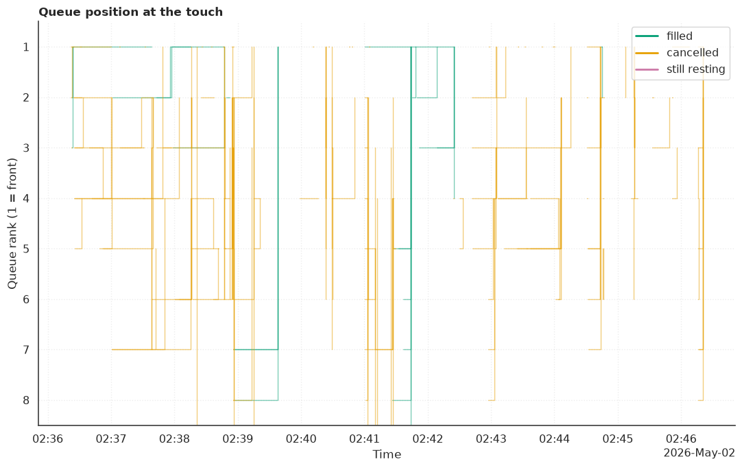
Filtered to the orders that ever reached the top five ranks — the front of the line, where fills happen — this is the same pattern as Ivy's fifty seconds, on real data: trajectories stepping downward as the queue ahead of them fills or cancels, then ending in a fill (×), a cancellation (○), or the window's edge.
Pitfall: not every L3 feed is a matched book
LOBSTER and exchange MBO feeds are matched books: the venue's
own engine guarantees bids never cross asks. The Bitstamp public
feed reconstructed here is a placement/cancellation diff
stream — and it genuinely contains crossed resting orders
(on the bundled sample, most of the crossed time comes from one
order that stays in the book long after it has left the venue;
the second exercise below finds it). order_book() replays such feeds
faithfully rather than silently "fixing" them: a crossed book in
your output is a property of the feed, not a reconstruction bug.
Know which kind of feed you're holding before you trust an
uncrossed-book invariant. The
Data quality explainer shows how to measure
the crossing (validate) and, if you must, uncross it for display.
Exercises
Try each one before you open its solution. Each solution runs when the documentation is built, so the answers are checked against this version of the library.
Exercise 1: where does a new order queue?
A new trader, Jo, posts a bid of 1 lot at 99 at t=10. Before you run anything, answer:
- What is Jo's queue rank at 99 when the bid arrives, and how many lots are ahead of it?
- Sam sells 3 lots at t=56. How much of Jo's bid fills?
- Now move Jo's bid to 100. What changes in Sam's sweep?
Write the session with toy_orders() and match_toy_orders (see
Change the script), then check
your answers with queue_positions(events, levels="all") from
ob_analytics.queue and the trades. queue_positions needs the classified
events, as order_book does: classify them with set_order_types first.
Solution
from ob_analytics import ToyOrder, match_toy_orders, toy_orders
from ob_analytics.analytics import set_order_types
from ob_analytics.queue import queue_positions

orders = toy_orders()
orders["Jo"] = ToyOrder(at=10, direction="bid", price=99, volume=1)
jo_events, jo_trades = match_toy_orders(orders)
jo_id = jo_events.loc[jo_events["actor"] == "Jo", "id"].iloc[0]
queue = queue_positions(set_order_types(jo_events, jo_trades), levels="all")
jo_queue = queue[queue["id"] == jo_id]
print(jo_queue[["price", "rank", "ahead_volume"]].to_string(index=False))
print()
sweep = jo_trades[jo_trades["taker_actor"] == "Sam"]
print(sweep[["price", "volume", "maker_actor"]].to_string(index=False))
assert jo_queue["rank"].iloc[0] == 3 and jo_queue["ahead_volume"].iloc[0] == 4
assert "Jo" not in set(sweep["maker_actor"])
 price  rank  ahead_volume
    99     3             4

 price  volume maker_actor
    99       2       Alice
    99       1         Ivy
Jo joins the back of the 99 queue: rank 3, behind Alice and Ivy, with their 4 lots ahead. Sam's 3 lots fill Alice's 2 and 1 of Ivy's, and stop before they reach Jo, so nothing of Jo's bid fills.
orders["Jo"] = ToyOrder(at=10, direction="bid", price=100, volume=1)
jo_events, jo_trades = match_toy_orders(orders)
sweep = jo_trades[jo_trades["taker_actor"] == "Sam"]
print(sweep[["price", "volume", "maker_actor"]].to_string(index=False))
assert list(sweep["maker_actor"]) == ["Jo", "Alice"]
 price  volume maker_actor
   100       1          Jo
    99       2       Alice
At 100 Jo's bid is alone at a better price, so it is first in line from t=10, although Alice and Ivy arrived earlier: price comes before time. Sam fills Jo at 100, then Alice's 2 lots at 99, and Ivy gets nothing. One tick bought Jo the front of the queue, which is the trade-off Hana faced: pay more, or wait.
Exercise 2: find the order that crosses the book
The pitfall above says the Bitstamp sample's book is crossed. Find the order responsible: which side it rests on, at what price, and how long it holds the touch after the venue no longer has it.
Hint: a matching engine fills the better price first, so a trade that
prints through a resting order shows that the order has already
left the venue. detect_stale_orders from ob_analytics.analytics
lists the orders the feed never removed after such a trade, worst
first.
Solution
from ob_analytics.analytics import detect_stale_orders

worst = detect_stale_orders(result.events, result.trades)[0]
print(f"side:            {worst.direction}")
print(f"price:           {worst.price:,.2f}")
print(f"disproved at:    {worst.disproved_at:%H:%M:%S}")
print(f"held the touch:  {worst.touch_seconds / 60:.1f} minutes")
assert worst.direction == "ask" and worst.touch_seconds > 20 * 60
side:            ask
price:           78,333.00
disproved at:    02:38:54
held the touch:  27.4 minutes
One ask, at 78,333.00. It came from the opening snapshot of the book. Trades printed above it about two and a half minutes into the capture, so it had already gone from the venue, but the feed never reported it again. It then held the ask touch for about 27 minutes, nearly the whole capture, and that one order is why the faithful book is crossed for most of the session. The Data quality explainer shows the crossed share of the session falling from about 92% to about 1% once it is removed.
Next: Loading order data — where these feed differences become practical.
Vocabulary introduced here — Level 1 / Level 2 / Level 3, market-by-order, price–time priority, queue rank, matched book vs diff feed — lives in the Glossary.