Loading order data
Chapters 1 and
2 used frames that arrived ready-made:
toy_events() returned a tidy table, Pipeline().run(...) produced
314,000 more rows of the same shape. This chapter is about where they
come from — how raw venue files, in whatever format a venue uses,
become the canonical events and trades frames every later chapter
consumes.
The route is always the same:
flowchart LR
    SRC[(venue files)] --> LD[loader]
    LD --> EV[canonical events]
    SRC --> TS[trade source]
    TS --> TR[canonical trades]
    EV --> CL[classify]
    TR --> CL
    CL --> DP[depth + metrics]
A loader speaks one venue's dialect and translates it into the canonical events frame; a trade source does the same for executions; everything downstream — classification, depth, every plot in this tutorial — reads only the canonical frames and never learns which venue they came from. Learn the contract once, and every new data source becomes a small translation exercise.
The canonical contract
So what exactly must a loader produce? The columns you have been
reading since chapter 1 (id, timestamp, price, volume,
action, direction, fill, …) plus two semantic rules, easiest to
see on a single order. Here is every event for Bob — he posted 3 at
101, sold 1 to Frank at t=20, and sold his last 2 to Hana at t=48:
%matplotlib inline
from ob_analytics import toy_events, toy_trades

events = toy_events()
events[events["actor"] == "Bob"][
    ["event_id", "actor", "action", "direction", "price", "volume", "fill"]
]
| event_id | actor | action | direction | price | volume | fill | |
|---|---|---|---|---|---|---|---|
| 1 | 2 | Bob | created | ask | 101 | 3 | 0 |
| 7 | 8 | Bob | changed | ask | 101 | 2 | 1 |
| 14 | 15 | Bob | deleted | ask | 101 | 0 | 2 |
Read the last two columns as what remains and what just traded:
volumeis the order's outstanding size after the event — 3 on arrival, 2 after Frank's fill, 0 after Hana's fill. It is running state, not the event's size.fillis the executed delta at the event — 0, then 1, then 2; summingfillgives Bob's traded total of 3.
So a fully filled order ends its life in a deleted row with
volume == 0 and fill > 0. A cancellation ends differently. Here is
Dana, who posted 3 at 98 and cancelled the whole order at t=40:
events[events["actor"] == "Dana"][
    ["event_id", "actor", "action", "direction", "price", "volume", "fill"]
]
| event_id | actor | action | direction | price | volume | fill | |
|---|---|---|---|---|---|---|---|
| 4 | 5 | Dana | created | bid | 98 | 3 | 0 |
| 10 | 11 | Dana | deleted | bid | 98 | 3 | 0 |
Her final row carries the removed size in volume and fill == 0:
nothing traded; three units left the book. Same deleted action,
opposite ending — the two numbers, not the action word, tell you which
case you are reading.
These rules are a contract, and the package enforces it:
ob_analytics.schemas is the single source of
truth for the required columns, with validators that raise on
violation. One column, type, is added by the classifier rather than
the loader, so we run that first — the same one-liner as chapter 1:
from ob_analytics.analytics import set_order_types
from ob_analytics.schemas import validate_events_df, validate_trades_df

events = set_order_types(events, toy_trades())  # adds `type` (chapter 1)
validate_events_df(events)
validate_trades_df(toy_trades())
print("both frames satisfy the contract")
both frames satisfy the contract
No news is good news — the validators return silently and raise
ConfigError the moment a required column is missing. And that is the
entire definition of a loader: any object whose load() returns
frames that pass these validators is a loader. No base class, no
registration, nothing else to implement. The
Custom components recipe builds one
for a made-up CSV dialect in about thirty lines.
Real data: the pipeline
For the two dialects the package ships, the translation is already written. The bundled ~30-minute Bitstamp BTC/USD capture loads with the exact call chapters 1 and 2 used:
from ob_analytics import Pipeline, sample_csv_path

result = Pipeline().run(sample_csv_path())
result.events.shape, result.trades.shape
((314057, 13), (284, 10))
One line hides a handful of canonical stages — load events, attach
trades, classify orders, compute depth and its summary metrics — each
an ordinary class you can also run by hand when you want the
intermediates (Step-by-step control).
Two conventions worth knowing: you point the pipeline at the orders
file and it resolves the companion trades.csv sitting next to it
automatically; and the result carries all four canonical frames
(events, trades, depth, depth_summary) plus the config that
produced them.
LOBSTER without leaving home
The other shipped dialect is LOBSTER — the academic standard for equity order-book data, the "premium L3 product" from chapter 2's table. A LOBSTER session is a pair of headerless CSVs: a message file (one row per order event) and an orderbook file (the top of the book after every message). There is no separate trades file — executions are message rows like everything else.
You may not have a session on disk. The package's writers are its loaders run in reverse, so we can write the toy session out as LOBSTER files and study the format on data we already know.
One translation first. LOBSTER does not say created / changed /
deleted; it numbers its event types — 1 = submission, 2 = partial
cancel, 3 = deletion, 4 = execution of visible liquidity, 5 =
execution of hidden liquidity (6 and 7, cross trades and halts, won't
appear here). And its size column is the per-event delta, not our
running volume. Both translations fall straight out of the
contract's two rules: any row with fill > 0 is an execution and the
fill is its delta; created rows are submissions; everything left in
this session is a cancellation.
import numpy as np

lob = events.copy()
lob["raw_event_type"] = np.where(
    lob["fill"] > 0, 4, np.where(lob["action"] == "created", 1, 3)
)
lob["raw_size"] = np.where(lob["fill"] > 0, lob["fill"], lob["volume"])
lob[["actor", "action", "volume", "fill", "raw_event_type", "raw_size"]].iloc[6:11]
| actor | action | volume | fill | raw_event_type | raw_size | |
|---|---|---|---|---|---|---|
| 6 | Frank | created | 1 | 0 | 1 | 1 |
| 7 | Bob | changed | 2 | 1 | 4 | 1 |
| 8 | Frank | deleted | 0 | 1 | 4 | 1 |
| 9 | Gus | created | 2 | 0 | 1 | 2 |
| 10 | Dana | deleted | 3 | 0 | 3 | 3 |
(These two columns, raw_event_type and raw_size, are exactly what
LOBSTER-born frames carry natively; we just retrofitted them onto a
Bitstamp-convention frame.) Now write the pair. Two LOBSTER-isms live
in the call: prices become integers in ten-thousandths of a dollar
(price_divisor=10_000), and timestamps become seconds after
midnight, so the writer must be told which midnight
(trading_date). The toy book's canonical prices are integer ticks with
a tick_size of $1 (its levels are whole dollars), and its sizes are
integer lots with a lot_size of 1 (whole units), so we pass both — the
writer scales ticks and lots back through them. Leave lot_size out and
the config default of 1e-8 writes a size of 2 as 2e-08:
import tempfile
from pathlib import Path

from ob_analytics import PipelineConfig, RunContext, save_data
from ob_analytics.datasets import LOT_SIZE, TICK_SIZE

toy_config = PipelineConfig(
    price_divisor=10_000, tick_size=TICK_SIZE, lot_size=LOT_SIZE
)
outdir = Path(tempfile.mkdtemp())
save_data(
    {"events": lob, "trades": toy_trades()},
    outdir,
    fmt="lobster",
    config=toy_config,
    ctx=RunContext(trading_date="2026-01-05"),
    ticker="TOY",
    num_levels=2,
)
sorted(p.name for p in outdir.iterdir())
['TOY_2026-01-05_2_message.csv', 'TOY_2026-01-05_2_orderbook.csv']
Ticker, date, and level count baked into the filenames, message and
orderbook twins side by side — the same pairing convention real
LOBSTER downloads use. (We passed no depth table, so the writer
computes the depth from events the way the pipeline does, and writes
the orderbook file from it.) Here are the first eleven message rows:
18000.0,1,1,2.0,990000,1
18002.0,1,2,3.0,1010000,-1
18005.0,1,3,1.0,980000,1
18006.0,1,4,2.0,990000,1
18008.0,1,5,3.0,980000,1
18012.0,1,6,2.0,1020000,-1
18020.0,1,7,1.0,1010000,1
18020.0,4,2,1.0,1010000,-1
18020.0,4,7,1.0,1010000,1
18035.0,1,8,2.0,1030000,-1
18040.0,3,5,3.0,980000,1
Every encoding is visible in the raw text. Column 1 is the time in seconds after the venue's local midnight. The writer's default venue zone is New York, so Alice's t=0, 10:00 UTC, is 05:00 there: 18000.0 seconds. Column 2 is the event-type code: seven type-1 submissions, then at 18020 two type-4 executions — Frank's market buy from chapter 1 hitting Bob (their order ids, 7 and 2, are column 3) — then Gus, then Dana's type-3 cancellation at 18040. Column 4 is the size delta, column 5 the price (990000 = $99.00), column 6 the side: 1 = bid, −1 = ask. Notice Frank's "market" buy arrives as a limit priced at the ask — chapter 1's crossing-the-spread, visible in a raw file.
The orderbook twin answers "and what did the book look like?" after every one of those messages. Its sixth row is the book just after Erin's arrival:
1010000,3,990000,4,1020000,2,980000,4
Read it interleaved, best levels first: ask₁ 101 × 3, bid₁ 99 × 4, ask₂ 102 × 2, bid₂ 98 × 4 — the ladder you learned to draw in chapter 1, flattened to one row per event. When a real LOBSTER session loads, this file is used as ground-truth depth instead of replaying it from the messages.
Now the trip home. LobsterSource bundles the matching loader, trade
reader, and config defaults (that price_divisor, among others), and
needs the same date anchor to turn seconds-after-midnight back into
timestamps. Its default tick_size is a cent, the equity grid, so it
would read $99.00 back as 9900 ticks; passing the same toy_config
that wrote the files keeps the toy's whole-dollar ticks:
from ob_analytics import LobsterSource

rt = Pipeline(
    source=LobsterSource(),
    config=toy_config,
    ctx=RunContext(trading_date="2026-01-05"),
).run(outdir)
print("executed units, original frames :", events["fill"].sum())
print("executed units, after round trip:", rt.events["fill"].sum())
executed units, original frames : 14
executed units, after round trip: 14
(With the source's own defaults, Pipeline.from_source("lobster",
ctx=...) is the short spelling.) The toy's five trades total 7 units;
counted from both sides — maker fills plus taker fills — that is 14
units of executions, and all 14 survive the round trip.
One honest wrinkle: the message file we wrote contains ten type-4 rows for those five trades, because our canonical stream records both sides of every fill, while a venue's own LOBSTER file logs each execution once, against the resting order — so the round-tripped trades frame reports ten trades. Executed volume is side-agnostic, which is why we verified on it. The reconstructed book is identical either way:
import matplotlib.pyplot as plt
import pandas as pd

from ob_analytics.analytics import order_book
from ob_analytics.visualization import plot, prepare

t30 = events["timestamp"].iloc[0] + pd.Timedelta(seconds=30)
fig, (ax1, ax2) = plt.subplots(1, 2, figsize=(10, 4.2), sharey=True)
plot(
    "book_snapshot",
    level="L2",
    ax=ax1,
    **prepare.book_snapshot(order_book(events, tp=t30)),
)
ax1.set_title("original toy events", fontsize=10)
plot(
    "book_snapshot",
    level="L2",
    ax=ax2,
    **prepare.book_snapshot(order_book(rt.events, tp=t30)),
)
ax2.set_title("after the LOBSTER round trip", fontsize=10)
ax2.set_ylabel("")
ax2.legend().remove()
fig.tight_layout()
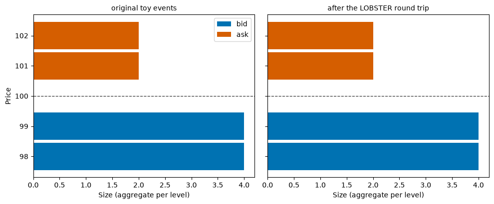
The same book at t=30, rebuilt from a different dialect. That is the promise of the canonical contract: once frames pass the validators, downstream code cannot tell — and does not care — where they came from.
Which loader path do you take?
Three routes into the canonical frames, in decreasing order of convenience:
| Your raw data | What you write | Recipe |
|---|---|---|
Bitstamp-format CSV capture (orders.csv + sibling trades.csv) |
Pipeline().run("run/orders.csv") |
Use your own data |
| LOBSTER message + orderbook files | Pipeline.from_source("lobster", ctx=RunContext(trading_date=...)).run(folder) |
Process LOBSTER files |
| Any other venue, API, or log | a small loader class whose load() returns validator-passing frames |
Custom components |
Whichever route you take, two warnings apply.
Pitfall: a LOBSTER file has no time zone
Timestamps in canonical frames are tz-aware UTC, whatever the
venue, so frames from different venues share one clock. A LOBSTER
file does not carry that clock: it stores seconds after the venue's
local midnight, with no zone. The writer and the loader place
those seconds with RunContext(session_tz=...), which defaults to
"America/New_York", the zone of LOBSTER's US equity data. We just
saw it: the toy's 10:00 UTC became 18 000 seconds, 05:00 in New
York. For a LOBSTER-format file from another venue, pass that
venue's zone both when you write and when you load. A wrong zone
moves every timestamp by whole hours, and nothing in the file shows
it.
Pitfall: know which kind of L3 file you hold
LOBSTER files come from a matched book (the venue's engine
guarantees bids never cross asks), while Bitstamp-style captures
are diff feeds that can genuinely contain crossed resting
orders — reread chapter 2's pitfall
and the glossary entry before you
trust an uncrossed-book invariant on reconstructed data. The
Data quality explainer shows how to measure
it with ob-analytics audit and clean it up with uncross=.
Next: Order lifecycles and classification — every order's history, from submission to one of four outcomes.
Vocabulary introduced here — Bitstamp CSV, LOBSTER, matched book vs diff feed — lives in the Glossary.