Order lifecycles and classification
Chapter 1 introduced the four order types as name-tags on the toy cast, and chapter 2 put "full order lifetimes" at the top of the list of things only L3 can answer. This chapter makes them the subject: every order has a history from placement to outcome, which the package recovers from the raw events — then classifies.
A lifecycle is two questions
In the events stream, every order's life follows one grammar:
flowchart LR
    C[created] -- "(changed) × N — fills and resizes" --> D[deleted]
    C -- "(changed) × N — never removed" --> S[survives the window]
Everything we can say about an order answers one of two questions about that arc — and the two are easy to conflate:
- Outcome: how did it end?
filled,cancelled, or stillrestingwhen the data ran out. - Type: how did it meet the spread along the way? Wait passively,
cross immediately, cross and then rest, or vanish untouched. This is
what
set_order_typesclassifies.
The axes are genuinely different. Alice and Chen have the same type
(resting-limit) but opposite outcomes (filled vs. still resting);
Alice and Hana share an outcome across different types. Keeping outcome
and type separate is half of reading any L3 analysis correctly.
Twelve orders, one table
order_lifecycles collapses the stream to one row per order — placed
when, at what price and size, how much filled, ended when and how. On
the toy session, with actors mapped back on and
times shown as seconds from the start:
%matplotlib inline
import pandas as pd

from ob_analytics import toy_events, toy_trades
from ob_analytics.analytics import order_lifecycles, set_order_types

events = set_order_types(toy_events(), toy_trades())
lc = order_lifecycles(events)
lc.insert(0, "actor", lc["id"].map(dict(zip(events["id"], events["actor"]))))
t0 = events["timestamp"].iloc[0]
lc["placed_s"] = (lc["placed_ts"] - t0).dt.total_seconds()
lc["end_s"] = (lc["end_ts"] - t0).dt.total_seconds()
lc[
    [
        "actor",
        "direction",
        "price",
        "placed_s",
        "placed_vol",
        "filled_vol",
        "end_s",
        "outcome",
        "type",
    ]
]
| actor | direction | price | placed_s | placed_vol | filled_vol | end_s | outcome | type | |
|---|---|---|---|---|---|---|---|---|---|
| 0 | Alice | bid | 99 | 0.0 | 2 | 2 | 56.0 | filled | resting-limit |
| 1 | Bob | ask | 101 | 2.0 | 3 | 3 | 48.0 | filled | resting-limit |
| 2 | Chen | bid | 98 | 5.0 | 1 | 0 | NaN | resting | resting-limit |
| 3 | Ivy | bid | 99 | 6.0 | 2 | 1 | NaN | resting | resting-limit |
| 4 | Dana | bid | 98 | 8.0 | 3 | 0 | 40.0 | cancelled | flashed-limit |
| 5 | Erin | ask | 102 | 12.0 | 2 | 0 | NaN | resting | resting-limit |
| 6 | Frank | bid | 101 | 20.0 | 1 | 1 | 20.0 | filled | market |
| 7 | Gus | ask | 103 | 35.0 | 2 | 0 | NaN | resting | resting-limit |
| 8 | Eve | bid | 100 | 45.0 | 1 | 0 | 45.8 | cancelled | flashed-limit |
| 9 | Hana | bid | 101 | 48.0 | 3 | 3 | 52.0 | filled | market-limit |
| 10 | Iris | ask | 101 | 52.0 | 1 | 1 | 52.0 | filled | market |
| 11 | Sam | ask | 99 | 56.0 | 3 | 3 | 57.0 | filled | market |
This is the chapter's anchor — every claim below traces back to a row here:
- Hana's whole chapter-1 sequence is one row: placed 3 at 101,
filled_vol3, typemarket-limit. She crossed for 2, rested 1, and the remainder was hit four seconds later; the row compresses all three steps. - Dana placed 3 and filled 0 — outcome
cancelled, and the classifier calls herflashed-limit, for reasons the next section makes precise. - Ivy filled 1 of her 2 and has an empty
end_s: its record has no end time. It is still open when the minute runs out, so its outcome isresting— a partial fill is not a complete one. - Frank and Iris appear and complete within a single second, and Sam's row spans just one (his sweep needed two prints): market orders leave lifecycle rows too, just very short ones.
What the classifier actually checks
set_order_types assigns the type column from two kinds of
evidence: the shape of the order's own events (created? deleted with
its size intact?) and what the trade tape records — every trade names the
event rows of its maker and taker (chapter 1's two roles) via
maker_event_id / taker_event_id.
| Type | The evidence | Toy cast |
|---|---|---|
resting-limit |
never crossed: survived the window untouched, or traded purely as a maker | Alice, Bob, Chen, Ivy, Erin, Gus |
market |
traded purely as a taker: crossed on arrival, never rested | Frank, Iris, Sam |
market-limit |
taker and maker: crossed, and the remainder rested | Hana |
flashed-limit |
created, then deleted with its full size intact — zero fills, at any lifetime | Dana, Eve |
pre-existing |
first seen mid-stream: no created row, no trades — the order predates the data |
— |
unknown |
none of the evidence patterns match | — |
Recall chapter 1's pitfall: flashed means unfilled, not fast. The rule compares the created and deleted sizes and never consults the clock, so Dana's 32 seconds and Eve's 800 ms flash earn the same label.
The last two rows are empty on the toy, and that is the point: a
hand-written session has no edges. pre-existing is not a
classification failure — an order already resting when the recording
begins is structurally unclassifiable, and the classifier says so
rather than guessing. unknown is the label for the rare event shapes
that fit no rule. Real captures have pre-existing orders, as we will
see shortly.
Lifespans as a picture
The lifecycle table has a natural picture, the order_activity face
at L3: each order one horizontal bar at its price, from placement to
outcome — green filled, orange cancelled, pink still resting, line width
proportional to size. The ladders below anchor it: the book as it
stood at four decisive instants, so every lifeline's start and end
can be checked against a state you can read directly:
from _docs_theme import plot_lifecycle_story

fig = plot_lifecycle_story(events, toy_trades(), at_s=[6, 40, 46, 57])
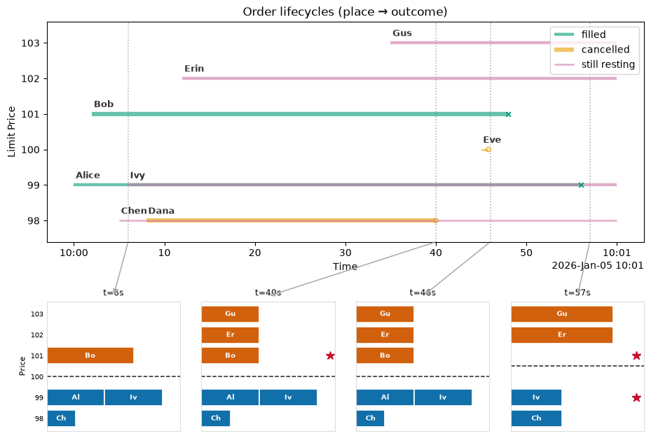
Eight lifelines, three endings — walking it top to bottom:
- Gus (103) and Erin (102) run pink to the right edge: placed, never touched, still resting at the end.
- Bob (101) is green: his 46-second bar ends in a × when Hana's crossing consumes his last 2 units.
- Eve (100) is the shortest bar on the plot — an 800 ms fleck that is nearly all ○.
- At 99 the face overprints: Alice and Ivy queued at the same price, so their lifelines share a lane. The clean green stub before t=6 is Alice alone; from Ivy's arrival the two blend; the × at t=56 is Alice's fill, and the pink that outlives it is Ivy. This face trades legibility for per-order identity — chapter 1's keyframes showed the queue; this shows the durations.
- At 98, Dana's thick orange bar (3 lots) ends in a ○ at t=40, while Chen's thin pink line — overprinted on top of it from t=5 — carries on to the edge alone.
And four actors are missing by design: the face draws the passive
classes only (resting- and flashed-limit). Frank, Iris and Sam live on
the trade tape, not in the book; Hana classified market-limit, so
even her four resting seconds are excluded. Chapter 2's lesson again:
know what a face excludes.
The running thread, at scale
Now put the same questions to the ~30-minute Bitstamp BTC/USD capture
— ~314,000 events, one pipeline run, and one type per order:
from ob_analytics import Pipeline, sample_csv_path
from ob_analytics.visualization import display_result

result = Pipeline().run(sample_csv_path())
# Canonical prices are integer ticks (issue #155); show quote currency.
result = display_result(result)
per_order = result.events.groupby("id")["type"].first()
summary = per_order.value_counts().to_frame("orders")
summary["share"] = (summary["orders"] / summary["orders"].sum()).map("{:.2%}".format)
summary
| orders | share | |
|---|---|---|
| type | ||
| flashed-limit | 156493 | 99.74% |
| resting-limit | 226 | 0.14% |
| market | 168 | 0.11% |
| pre-existing | 13 | 0.01% |
| market-limit | 2 | 0.00% |
| unknown | 0 | 0.00% |
The proportions are nothing like the toy's. Of roughly 157,000 orders,
about 99.7% classify flashed-limit — created and cancelled,
never filled. The two crossing classes together are barely a tenth of
a percent: about one order in a thousand arrives intending to trade
immediately. Chapter 1 treated Eve's flash as the exotic case; at
scale, Eve is the overwhelming norm, and it is Alice — post, wait,
fill — who is rare. The pre-existing class the toy couldn't produce
is here too, in tiny numbers. unknown stays empty: every order in
this sample fits one of the rules.
import matplotlib.pyplot as plt

fig, ax = plt.subplots(figsize=(9, 3.4))
ax.bar(summary.index.astype(str), summary["orders"], color="#1170aa")
ax.set_yscale("log")
ax.set_ylim(1, summary["orders"].max() * 12)
ax.bar_label(ax.containers[0], fmt="{:,.0f}", padding=2)
ax.set_ylabel("orders (log scale)")
ax.set_title("Order classes in the sample capture")
Text(0.5, 1.0, 'Order classes in the sample capture')
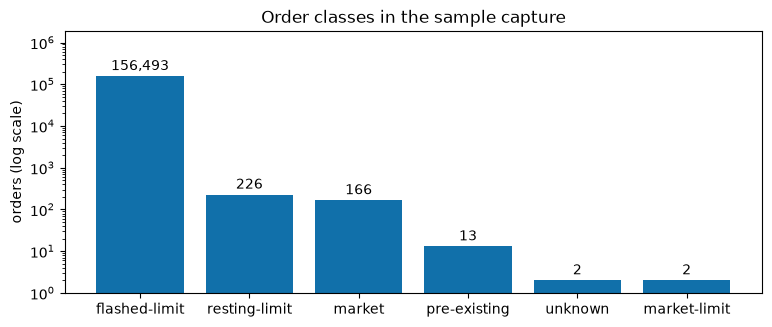
The axis is logarithmic because it has to be: on a linear scale the flashed-limit column — nearly 400× everything else combined — would be the only visible bar.
Why would anyone behave like this? Because a resting quote at a stale price is a free option for everyone else. Modern liquidity provision is algorithmic quote management: as the fair price drifts, market-making systems cancel and repost their quotes to follow it — and on a venue where order ids are not reusable, every one of those updates is a fresh order that lives briefly and dies unfilled. The lifetimes carry the signature:
lc_real = order_lifecycles(result.events)
fl = lc_real[lc_real["type"].astype(str) == "flashed-limit"].copy()
end = result.events["timestamp"].max()
fl = fl[
    fl["end_ts"] <= end - pd.Timedelta(seconds=2)
]  # drop the shutdown burst (next section)
life = (fl["end_ts"] - fl["placed_ts"]).dt.total_seconds()
{f"under {t}s": f"{(life < t).mean():.1%}" for t in (1, 10, 60)}
{'under 1s': '89.2%', 'under 10s': '96.4%', 'under 60s': '99.3%'}
Roughly nine in ten flashed orders live under a second; nineteen in twenty are gone within ten. At ~90 order placements per second against a few hundred trades in the whole half hour, this book is not a queue of patient humans — it is a handful of algorithms continuously retyping their prices. Eve is the norm because in per-order data, a quote update is a brief, unfilled order.
Outcomes show the same pattern from the other axis:
outcome
cancelled    156495
filled          302
partial          92
Name: count, dtype: int64
Now look closely at the edges, because two of these numbers should
bother you. First, 13 orders classify pre-existing: deletions whose
creations happened before the recording started — the window's leading
edge (it would be thousands, but this capture's collector opens with a
book snapshot, emitting synthetic created rows for every order
already standing). Second, only one order out of ~157,000 is still
resting at the end. After thirty minutes, a real book holds
thousands of standing orders — where did they go?
end = result.events["timestamp"].max()
deletes = result.events[result.events["action"] == "deleted"]
deletes[deletes["timestamp"] > end - pd.Timedelta(seconds=2)]["id"].nunique()
6624
They were closed by the recorder. This capture was made with the
package's own live collector, which — by its documented convention —
closes every lifecycle at shutdown, emitting a synthetic deleted
for each order still standing so that no id is left dangling. The
receipts ship with the sample: its meta.json records
synthetic_deleted: 6518, and that is the ~6,600-deletion burst we
just measured in the final two seconds, against a baseline of one or
two hundred per second.
This is a property of the collector, not of order books. A
capture made by a recorder without that convention would end with
thousands of orders whose fate is resting — and a correspondingly
smaller flashed-limit count, since each synthetically closed order
now carries a created-then-cancelled-unfilled shape that the
classifier — correctly, on the evidence it has — calls
flashed-limit. (In this capture that accounts for about 6,500 of
the 156,000 flashed orders — the repricing churn above, not the
shutdown, dominates.) The recorder's conventions are part of the
window. We return to this in the pitfall at the end of the chapter.
One picture of all those endings at once — each order plotted at the size it was placed and where it was placed relative to the best quote (in basis points; the measure the next section unpacks), colored by outcome:
from ob_analytics.visualization import plot, prepare

fig = plot("order_outcome", level="L3", **prepare.order_outcome_l3(result.events))
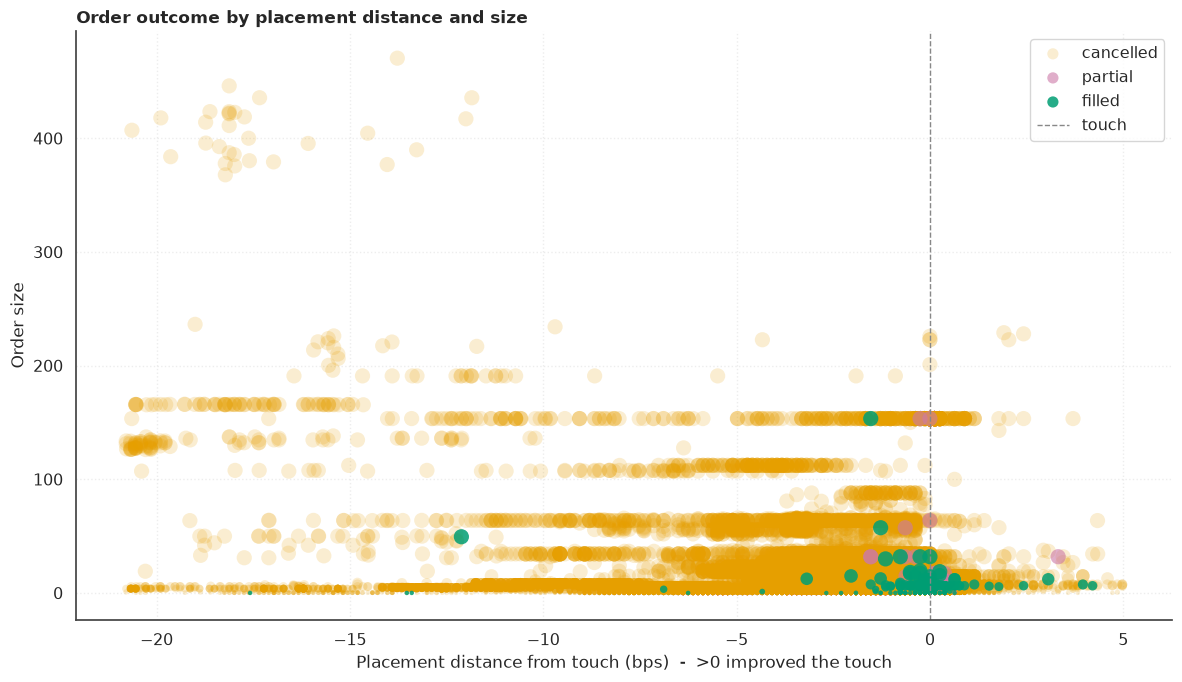
The green fills cluster at the dashed touch line while the orange cancellations spread away from it, at every size: where you stand, not how big you are, decides whether you trade.
Aggressiveness: the continuous version of the classes
The four classes are discrete answers to "how did it meet the
spread?". order_aggressiveness asks the same question continuously:
at the moment of placement, how far was the order from the best quote
on its own side, in basis points — positive means it improved the
touch, negative means it queued behind it. Back to the toy for the
last time:
from ob_analytics.analytics import order_aggressiveness
from ob_analytics.depth import depth_metrics, price_level_volume

agg = order_aggressiveness(events, depth_metrics(price_level_volume(events)))
placed = agg[agg["action"] == "created"].set_index("actor")
placed[["price", "type", "aggressiveness_bps"]].round(1)
| price | type | aggressiveness_bps | |
|---|---|---|---|
| actor | |||
| Alice | 99 | resting-limit | NaN |
| Bob | 101 | resting-limit | NaN |
| Chen | 98 | resting-limit | -101.0 |
| Ivy | 99 | resting-limit | 0.0 |
| Dana | 98 | flashed-limit | -101.0 |
| Erin | 102 | resting-limit | -99.0 |
| Frank | 101 | market | NaN |
| Gus | 103 | resting-limit | -198.0 |
| Eve | 100 | flashed-limit | 101.0 |
| Hana | 101 | market-limit | NaN |
| Iris | 101 | market | NaN |
| Sam | 99 | market | NaN |
- Eve, +101 bps: her bid at 100 stood a full percent above the best bid of 99 — the session's most aggressive passive placement (chapter 1 watched it drag the mid up).
- Ivy, 0.0: joined the queue exactly at the best — the market-maker's default.
- Chen and Dana, −101: one price level behind the touch; Erin (−99) and Gus (−198): one and two levels back on the ask side.
- Alice and Bob get no number: each was the first order on their
side of the book, so there was no prevailing quote to measure
against — Alice's
NaN, and Bob's degenerate-inf(the empty ask side as reference), which the plotting faces drop before drawing. - Frank, Hana, Iris and Sam get no number by design: the measure is computed for the passive classes only. Crossing orders already answered the question categorically — they were maximally aggressive.
In one line: the classes say whether an order crossed; aggressiveness says where it chose to stand when it didn't. It is the x-axis of the outcome scatter above — the continuous refinement of the discrete taxonomy.
Pitfall: the window and the tape
Everything in this chapter rests on two inputs: the event window (when the recording starts and stops) and the trade tape (whether fills can be attributed to orders). "Dana is a flashed-limit order" sounds like a property of Dana. It is not — it is a property of Dana as seen through this window, with this tape. The experiment is cheap: replay the toy as if the recording had started at t=12 (the first five events lost), then replay that late window again with the trade feed unplugged:
def classify(ev, tr):
    return set_order_types(ev, tr).groupby("actor", observed=True)["type"].first()


late_events = toy_events().iloc[5:]  # recording now starts at t=12
pd.DataFrame(
    {
        "full window": classify(toy_events(), toy_trades()),
        "late window": classify(late_events, toy_trades()),
        "late window, no tape": classify(late_events, toy_trades().iloc[:0]),
    }
)
| full window | late window | late window, no tape | |
|---|---|---|---|
| actor | |||
| Alice | resting-limit | resting-limit | pre-existing |
| Bob | resting-limit | resting-limit | pre-existing |
| Chen | resting-limit | NaN | NaN |
| Dana | flashed-limit | pre-existing | pre-existing |
| Erin | resting-limit | resting-limit | resting-limit |
| Eve | flashed-limit | flashed-limit | flashed-limit |
| Frank | market | market | unknown |
| Gus | resting-limit | resting-limit | resting-limit |
| Hana | market-limit | market-limit | unknown |
| Iris | market | market | unknown |
| Ivy | resting-limit | resting-limit | pre-existing |
| Sam | market | market | unknown |
Column by column, left to right:
- Full window — the twelve familiar labels.
- Late window — Dana flips to
pre-existing: same order, same cancellation, but hercreatedrow now predates the recording, so the evidence forflashed-limitis gone. Chen vanishes entirely (his creation was his only event): an order can be not just unclassifiable but invisible. Alice, Bob and Ivy, who also lost theircreatedrows, keepresting-limit— the tape rescues them, because their fills name them as makers. - Late window, no tape — the rescue is revoked: Alice, Bob and Ivy
sink to
pre-existing, and Frank, Hana, Iris and Sam — the orders that actually traded — collapse tounknown. When a venue's trades cannot be matched to its events, it is precisely the trading orders whose classes degrade.
Pitfall: classification is a property of the window and the tape, not of the order
The same Dana is flashed-limit in one capture and pre-existing
in a capture that starts twelve seconds later; the same Frank is
market with a matched tape and unknown without one. Before
comparing class proportions across captures — or trusting them
within one (recall the shutdown drain above) — ask when the window
starts and ends, and whether the venue's trades carry usable
maker_event_id / taker_event_id attribution. Neither
pre-existing nor unknown is a bug; both are the classifier
refusing to invent evidence it does not have.
Exercise: what if Eve had not flashed?
Eve posts a bid of 1 lot at 100 at t=45 and cancels it 800 ms later. Suppose she leaves it in the book. Before you run anything, predict:
- Which orders does Sam's sell of 3 lots at t=56 fill, and at which prices?
- Eve's outcome and type.
- Ivy's outcome, and how much of her bid fills.
Write the session with toy_orders() and match_toy_orders (see
Change the script);
dataclasses.replace(orders["Eve"], cancel_at=None) removes the
cancellation. Then check your predictions with set_order_types and
order_lifecycles, as at the start of the chapter.
Solution
from dataclasses import replace

from ob_analytics import match_toy_orders, toy_orders

orders = toy_orders()
orders["Eve"] = replace(orders["Eve"], cancel_at=None)
eve_events, eve_trades = match_toy_orders(orders)
eve_events = set_order_types(eve_events, eve_trades)
sweep = eve_trades[eve_trades["taker_actor"] == "Sam"]
print(sweep[["price", "volume", "maker_actor"]].to_string(index=False))
print()
eve_lc = order_lifecycles(eve_events)
eve_lc.insert(
    0, "actor", eve_lc["id"].map(dict(zip(eve_events["id"], eve_events["actor"])))
)
eve_lc = eve_lc.set_index("actor").loc[["Eve", "Alice", "Ivy"]]
print(eve_lc[["placed_vol", "filled_vol", "outcome", "type"]].to_string())
assert list(sweep["maker_actor"]) == ["Eve", "Alice"]
assert eve_lc.loc["Eve", "type"] == "resting-limit"
assert eve_lc.loc["Ivy", "filled_vol"] == 0
 price  volume maker_actor
   100       1         Eve
    99       2       Alice

       placed_vol  filled_vol  outcome           type
actor
Eve             1           1   filled  resting-limit
Alice           2           2   filled  resting-limit
Ivy             2           0  resting  resting-limit
When Sam arrives, Eve's bid at 100 is the best bid: Hana's last lot at 101 was taken by Iris at t=52. So Sam fills Eve first, at 100, then Alice's 2 lots at 99, and his 3 lots are gone before Ivy's turn.
Eve's outcome becomes filled and her type resting-limit: the same
order, placed at the same time, changes class because of how it ended.
flashed-limit describes what happened to an order, not what its
owner meant to do. Ivy, half-filled in the original session, now ends
resting with nothing filled: one order that stayed in the book
changed the outcome of an order behind it in the queue.
Next: Depth, spread and liquidity — from individual orders to aggregate depth.
Vocabulary introduced here — resting-limit / market / market-limit / flashed-limit, maker / taker, basis point, order lifecycle, outcome (filled / cancelled / resting), pre-existing, unknown, placement aggressiveness — lives in the Glossary.