Trades and flow toxicity
Chapters 4 and 5 were about supply — the orders standing in the book, who placed them, how much rests where. This chapter is about demand: the trades that cross the spread and consume that supply, and a question every liquidity provider cares about — is this flow toxic?
"Toxic" has a precise meaning. When you post a resting quote, you are writing a free option: anyone may trade against you at your price. Usually that is fine — you collect the spread from impatient traders who have no special information. But sometimes the person hitting your quote knows something you don't (a fill is coming, a number is about to print), and the price is about to move against you. Flow from informed traders is toxic — it systematically loses you money — and three classic measures try to detect it from the trade tape alone. We will meet each the same way: the formula, what it means in one sentence, its source, then the code — on a tape small enough to check by hand.
A constructed tape
The toy order book had only five trades — flow metrics are built for thousands, so we construct a busier tape with a deliberate arc: a calm, balanced open; then an informed buyer accumulates, lifting the price from 100 to 103; then calm again at the new level. Every metric below should rise in the middle and stay low at the edges.
%matplotlib inline
import matplotlib.pyplot as plt
import pandas as pd
from _docs_theme import ASK_COLOR, BID_COLOR

base = pd.Timestamp("2026-01-05 10:00:00")
_t = []


def trade(sec, price, volume, side):
    _t.append(
        {
            "timestamp": base + pd.Timedelta(seconds=sec),
            "price": float(price),
            "volume": float(volume),
            "direction": side,
        }
    )


# calm: balanced buys and sells at 100
trade(0, 100, 2, "buy")
trade(10, 100, 2, "sell")
trade(20, 100, 2, "buy")
trade(30, 100, 2, "sell")
# informed accumulation: a run of buys walks the price up
trade(60, 100, 4, "buy")
trade(70, 101, 4, "buy")
trade(80, 101, 4, "buy")
trade(90, 102, 4, "buy")
trade(100, 103, 4, "buy")
# calm again at the new level
trade(130, 103, 2, "sell")
trade(140, 103, 2, "buy")
trade(150, 103, 2, "sell")
trade(160, 103, 2, "buy")

tape = pd.DataFrame(_t)
tape["direction"] = pd.Categorical(tape["direction"], categories=["buy", "sell"])


def draw_tape(ax):
    """The reference tape: price over time, buys green-up, sells orange-down,
    marker area ~ volume, the accumulation window shaded."""
    ax.axvspan(
        base + pd.Timedelta(seconds=45),
        base + pd.Timedelta(seconds=115),
        color="#f2e6c9",
        alpha=0.6,
        zorder=0,
    )
    for side, color, marker in (("buy", BID_COLOR, "^"), ("sell", ASK_COLOR, "v")):
        s = tape[tape["direction"] == side]
        ax.scatter(
            s["timestamp"],
            s["price"],
            s=s["volume"] * 40,
            c=color,
            marker=marker,
            edgecolor="white",
            linewidth=0.6,
            zorder=3,
            label=side,
        )
    ax.plot(tape["timestamp"], tape["price"], color="#888", lw=0.8, zorder=1)
    ax.set_ylabel("Trade price")
    ax.legend(loc="upper left", framealpha=0.9)


fig, ax = plt.subplots(figsize=(11, 3.6))
draw_tape(ax)
ax.set_title("The reference tape — informed accumulation shaded")
Text(0.5, 1.0, 'The reference tape — informed accumulation shaded')
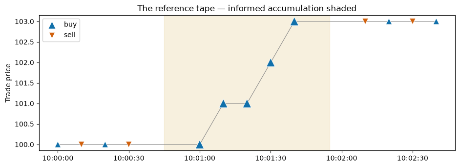
Thirteen trades: four calm, five in the shaded accumulation, four calm again. Three buckets, three metrics, one tape.
Order flow imbalance: the direction of the flow
The simplest measure. Over a time window, net the buy and sell volume and normalise:
In one sentence: OFI is which way the flow leaned, on a scale from −1 (everyone sold) through 0 (balanced) to +1 (everyone bought). It is the short-horizon pressure on price, and it is a simpler relative of the order-book event imbalance studied by Cont, Kukanov and Stoikov (2014). On the tape, in 30-second windows:
from ob_analytics.flow_toxicity import order_flow_imbalance

ofi = order_flow_imbalance(tape, window="30s")
ofi[["timestamp", "buy_volume", "sell_volume", "ofi"]]
| timestamp | buy_volume | sell_volume | ofi | |
|---|---|---|---|---|
| 0 | 2026-01-05 10:00:00 | 4.0 | 2.0 | 0.333333 |
| 1 | 2026-01-05 10:00:30 | 0.0 | 2.0 | -1.000000 |
| 2 | 2026-01-05 10:01:00 | 12.0 | 0.0 | 1.000000 |
| 3 | 2026-01-05 10:01:30 | 8.0 | 0.0 | 1.000000 |
| 4 | 2026-01-05 10:02:00 | 2.0 | 2.0 | 0.000000 |
| 5 | 2026-01-05 10:02:30 | 2.0 | 2.0 | 0.000000 |
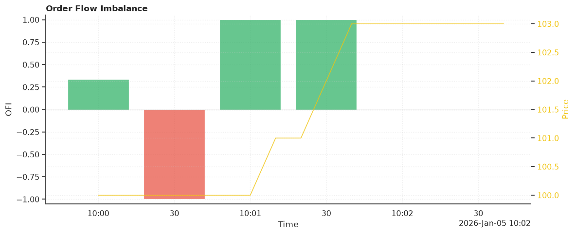
Read it against the tape above: the two calm-open windows are +0.33
and −1.0 (small, mixed), the two accumulation windows peg at +1.0
(buys only), and the calm close settles back to 0.0. The ofi face
draws exactly this, the tape on top and the imbalance bars below —
note how the bars swell and turn one-sided precisely under the shaded
region:
from ob_analytics.visualization import plot, prepare

fig = plot("order_flow_imbalance", **prepare.ofi(ofi, trades=tape))
VPIN: imbalance on a volume clock
OFI slices time into equal minutes. VPIN — Volume-Synchronised
Probability of Informed Trading — slices into equal volume instead,
which is the key idea. Markets trade in bursts; a volume clock
ticks fast when trading is frenzied and slow when it
is quiet, so each bucket carries the same economic weight. Within each
bucket of V units, VPIN measures the same imbalance:
In one sentence: VPIN is the average one-sidedness of trading per unit of volume — high when buyers and sellers are lopsided, which is the footprint of someone trading on information (Easley, López de Prado and O'Hara, 2012). Note the absolute value: VPIN does not care which side is winning, only that the flow is imbalanced. With 8-unit buckets:
from ob_analytics.flow_toxicity import compute_vpin

vpin = compute_vpin(tape, bucket_volume=8.0, n_buckets=3)
vpin[["bucket", "buy_volume", "sell_volume", "vpin", "vpin_avg"]].round(3)
| bucket | buy_volume | sell_volume | vpin | vpin_avg | |
|---|---|---|---|---|---|
| 0 | 0 | 4.0 | 4.0 | 0.0 | 0.000 |
| 1 | 1 | 8.0 | 0.0 | 1.0 | 0.500 |
| 2 | 2 | 8.0 | 0.0 | 1.0 | 0.667 |
| 3 | 3 | 6.0 | 2.0 | 0.5 | 0.833 |
Bucket 0 gathers the calm open — 4 buys, 4 sells, imbalance
|4−4|/8 = 0. The accumulation buckets are 8 units of pure buying:
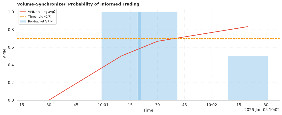
|8−0|/8 = 1. The headline number is vpin_avg, the trailing mean —
it climbs from 0 through the accumulation and decays afterward, a
smoothed toxicity measure. The face plots that climb, with a threshold
line above which flow is "toxic":
Kyle's λ: the price of a unit of flow
OFI and VPIN measure imbalance. Kyle's λ measures its consequence: how far the price moves per unit of net order flow. Over each window, take the price change and the signed volume, then fit a line across all windows:
In one sentence: λ is the price you pay per unit of net flow — the slope of price against signed volume, and the market's illiquidity, since in a deep liquid market even large imbalances barely nudge the price (Kyle, 1985). A big λ means a small trade moves the market a lot. Fitting on the tape:
from ob_analytics.flow_toxicity import compute_kyle_lambda

kyle = compute_kyle_lambda(tape, window="30s")
print(f"λ = {kyle.lambda_:.4f}   t = {kyle.t_stat:.2f}   R² = {kyle.r_squared:.3f}")
kyle.regression_df.round({"delta_price": 2, "signed_volume": 2})
λ = 0.0893 t = 5.77 R² = 0.893
| timestamp | delta_price | signed_volume | |
|---|---|---|---|
| 0 | 2026-01-05 10:00:00 | 0.0 | 2.0 |
| 1 | 2026-01-05 10:00:30 | 0.0 | -2.0 |
| 2 | 2026-01-05 10:01:00 | 1.0 | 12.0 |
| 3 | 2026-01-05 10:01:30 | 1.0 | 8.0 |
| 4 | 2026-01-05 10:02:00 | 0.0 | 0.0 |
| 5 | 2026-01-05 10:02:30 | 0.0 | 0.0 |
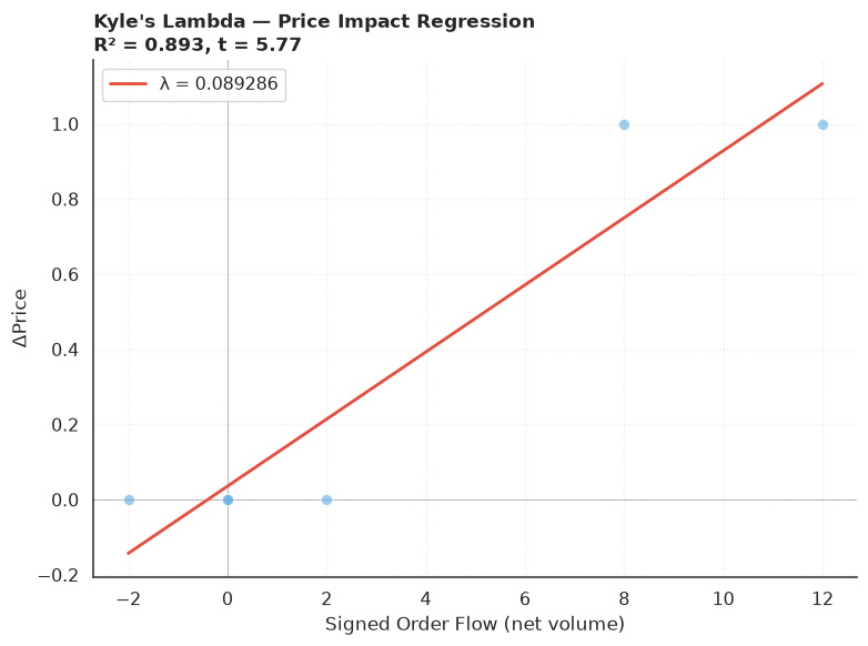
The regression table is the anchor: the two calm-open windows carry signed volume ±2 with no price change, while the accumulation windows carry +12 and +8 signed units and lift the price +1 each. A line through those points has slope λ ≈ 0.09 — about one price unit per eleven net units of flow — with a t-statistic near 6 and R² ≈ 0.89: on this constructed tape, signed flow explains nearly all of the price moves.
The result also says how far to trust that slope. diagnostics lists
the reasons not to, and significant is True only when the list is
empty:
significant: False
 - only 6 windows; at least 30 are needed for the fit to mean much
A t-statistic near 6 is not enough on its own: six windows are far too few for any regression, and the check says so. That is the right verdict for a tape built to be checked by hand, not to draw conclusions from. The face draws the scatter and its fitted line:
The same three metrics on real data
Now the running Bitstamp capture — the tape we have been building on since chapter 3, all 284 of its trades:
from ob_analytics import Pipeline, sample_csv_path
from ob_analytics.visualization import display_result

result = Pipeline().run(sample_csv_path())
# Canonical prices are integer ticks (issue #155); show quote currency.
result = display_result(result)
kyle_real = compute_kyle_lambda(result.trades, window="5min")
print(
    f"trades: {len(result.trades)}   total volume: {result.trades['volume'].sum():.1f}"
)
print(
    f"λ = {kyle_real.lambda_:.3f}   t = {kyle_real.t_stat:.2f}   "
    f"R² = {kyle_real.r_squared:.3f}   windows = {kyle_real.n_windows}"
)
print(
    f"{kyle_real.ci_level:.0%} interval: "
    f"[{kyle_real.ci_low:.3f}, {kyle_real.ci_high:.3f}]"
)
print(f"significant: {kyle_real.significant}")
for reason in kyle_real.diagnostics:
    print(" -", reason)
trades: 284   total volume: 15.0
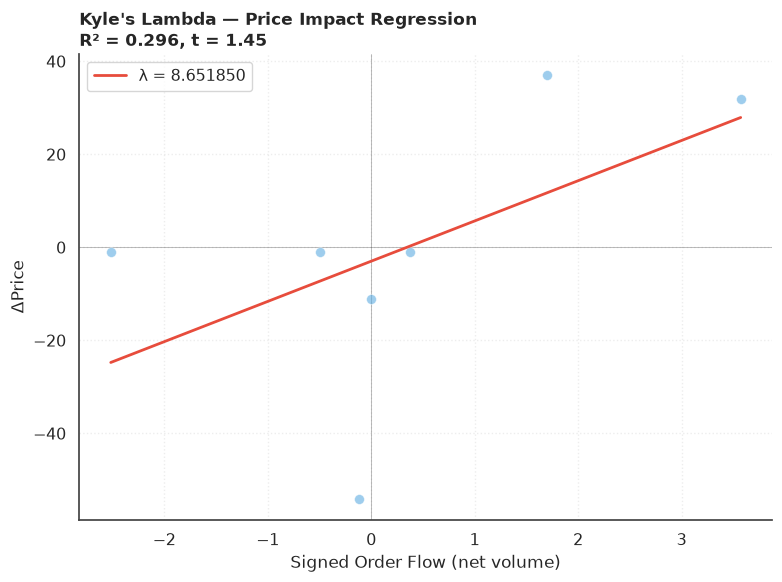
λ = 8.652   t = 1.45   R² = 0.296   windows = 7
95% interval: [-9.790, 18.528]
significant: False
 - only 7 windows; at least 30 are needed for the fit to mean much
 - |t| = 1.45 is below 2; λ is not distinguishable from zero
Look at the t-statistic before the λ: 1.45. As a rule of thumb a coefficient needs |t| ≳ 2 to be distinguishable from zero, so this λ — positive, but weak — is not statistically significant, and the result says so itself, along with the second reason: seven windows. The confidence interval makes the same point in λ's own units. It comes from a block bootstrap: resample runs of neighbouring windows with replacement, refit the slope each time, and keep the middle 95% of the slopes. The interval runs from below zero to above it, so the data cannot even settle the sign of λ.
VPIN reports the same kind of check. Leave bucket_volume out and it
is picked from the tape with the common rule, average daily volume ÷ 50.
A thirty-minute capture is scaled up to a day at the rate it traded, so
each bucket holds about half an hour of this tape's volume:
import warnings

# compute_vpin also raises a UserWarning here; suppressed since the
# diagnostics it points at are printed explicitly below.
with warnings.catch_warnings():
    warnings.simplefilter("ignore", UserWarning)
    vpin_real = compute_vpin(result.trades)
print(
    f"bucket_volume = {vpin_real.attrs['bucket_volume']:.2f} "
    f"({vpin_real.attrs['bucket_volume_rule']})   buckets = {len(vpin_real)}"
)
for reason in vpin_real.attrs["diagnostics"]:
    print(" -", reason)
bucket_volume = 14.51 (adv/50)   buckets = 1
 - only 1 complete bucket, fewer than n_buckets=50; vpin_avg never averages a full window
One bucket, where the trailing average wants fifty. That is the honest headline for this dataset: a quiet thirty-minute capture with 284 trades and fifteen units of total volume is far below the regime these metrics were designed for. They compute; they just cannot conclude — and now they say so.
Pitfall: these metrics need volume, and their knobs are not neutral
Flow-toxicity measures were built for high-frequency equity and
futures data — thousands of trades per minute, not a handful per
minute. On a thin tape, three problems arise. (1) Significance: as
above, λ's t-statistic collapses; VPIN's trailing average is taken
over too few buckets to mean much. Read significant and
diagnostics on the λ result, and attrs["diagnostics"] on the
VPIN frame, before the number. (2) The knobs move the
answer: bucket_volume for VPIN and window for Kyle and OFI
are not neutral defaults — halve the bucket size and VPIN's whole
profile shifts. Choose them from the instrument's typical volume
(vpin_bucket_volume applies the average daily volume ÷ 50 rule),
and report them alongside the number; the VPIN frame keeps its
bucket size in attrs["bucket_volume"] for this. (3) Trade side is itself an
inference: every metric here needs each trade labelled buy or
sell, which ob-analytics knows exactly (the taker's direction
from chapter 4) — but on venues that ship only anonymous prints
you must guess the side (the tick rule, Lee–Ready), and the
guess's errors flow straight into every metric on this page.
Metrics from a result, and metrics of your own
Everything above called the functions directly on a trades table. From
a pipeline result, the same measurements are also registered metrics:
each has a name, runs over the result, and draws as a plot.
result.metric(name) returns the table and result.plot(name) draws
it, with the function's defaults unless you pass a setting:
The registered names are vpin, kyle_lambda, order_flow_imbalance
and ofi_horizon, plus l1_ticker, the quote from chapter 1.
A flow metric is still just a function over a trades table. Here is
Amihud's (2002) illiquidity, |return| per unit volume, in four lines:
def amihud(trades: pd.DataFrame, freq: str = "30s") -> pd.DataFrame:
    t = trades.set_index("timestamp").sort_index()
    ret = t["price"].pct_change().abs()
    return (ret / t["volume"]).resample(freq).mean().rename("amihud").reset_index()


amihud(tape).dropna().round({"amihud": 5})
| timestamp | amihud | |
|---|---|---|
| 0 | 2026-01-05 10:00:00 | 0.00000 |
| 1 | 2026-01-05 10:00:30 | 0.00000 |
| 2 | 2026-01-05 10:01:00 | 0.00083 |
| 3 | 2026-01-05 10:01:30 | 0.00246 |
| 4 | 2026-01-05 10:02:00 | 0.00000 |
| 5 | 2026-01-05 10:02:30 | 0.00000 |
It rises in the accumulation windows for the same reason λ does —
price moving on volume. To make it a metric like the built-ins, wrap it
in a small class and register it with register_metric; it then shows
in available_concepts, draws with result.plot("amihud") and gets a
gallery card (see Extending ob-analytics).
The point of the whole chapter: these are ordinary functions over a
trades table, and on a small tape you can check every number by hand.
Exercise: move the VPIN bucket
The pitfall says bucket_volume is not a neutral setting. Test that on
the constructed tape, which holds 36 units of volume. Keep
n_buckets=3 and, before you run anything, predict for
bucket_volume=4 and bucket_volume=16:
- How many buckets does the tape fill?
- Does the peak
vpin_avgrise above or fall below the 0.833 it reaches with 8-unit buckets, and why?
Solution
rows = {}
for size in (4.0, 8.0, 16.0):
    # 16-unit buckets fill fewer than n_buckets, and compute_vpin warns.
    with warnings.catch_warnings():
        warnings.simplefilter("ignore", UserWarning)
        v = compute_vpin(tape, bucket_volume=size, n_buckets=3)
    rows[f"bucket_volume={size:g}"] = {
        "buckets": len(v),
        "one-sided buckets": int((v["vpin"] == 1).sum()),
        "peak vpin_avg": round(v["vpin_avg"].max(), 3),
    }
by_size = pd.DataFrame(rows).T
print(by_size.to_string())
assert by_size["buckets"].tolist() == [9, 4, 2]
assert by_size["peak vpin_avg"].tolist() == [1.0, 0.833, 0.625]
                  buckets  one-sided buckets  peak vpin_avg
bucket_volume=4       9.0                5.0          1.000
bucket_volume=8       4.0                2.0          0.833
bucket_volume=16      2.0                0.0          0.625
4 units: nine buckets, and the peak rises to 1.0. Each calm pair of trades fills one balanced bucket (VPIN 0), and the five 4-unit buys of the accumulation fill five buckets of pure buying (VPIN 1). Three of those in a row put the trailing average at 1.0, where it stays for three buckets before it falls back.
16 units: two buckets, and the peak falls to 0.625. Each bucket mixes calm trading with part of the accumulation, so neither is one-sided (0.5 and 0.75), and the informed run is diluted. With only two buckets, the average also covers fewer buckets than the three it was asked for.
The tape did not change; only the clock did. Smaller buckets show a short burst sharply, but each holds fewer trades, so on a real tape they are noisier. Larger buckets are steadier but can hide the burst. That is why a VPIN number means little without the bucket size beside it.
Next: The visualization system — the concepts, levels and backends behind every figure in this tutorial, and how to compose your own.
Vocabulary introduced here — flow toxicity, informed trading, VPIN, Kyle's lambda, order flow imbalance, volume clock — lives in the Glossary.